Time Series Data: Univariate, Multivariate, Panel, and Exogenous Variables
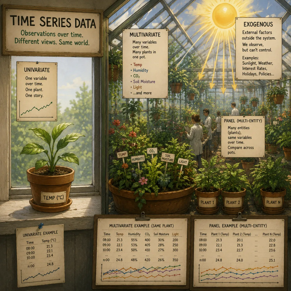
A practical guide to the main types of time series data and the common confusion between multivariate, panel, and exogenous-variable forecasting.
- forecasting
- multivariate
Section 4 of 8
Data preparation, forecasting models, deep learning, foundation models, evaluation, maintenance.
18 items in this section.
A practical guide to the main types of time series data and the common confusion between multivariate, panel, and exogenous-variable forecasting.
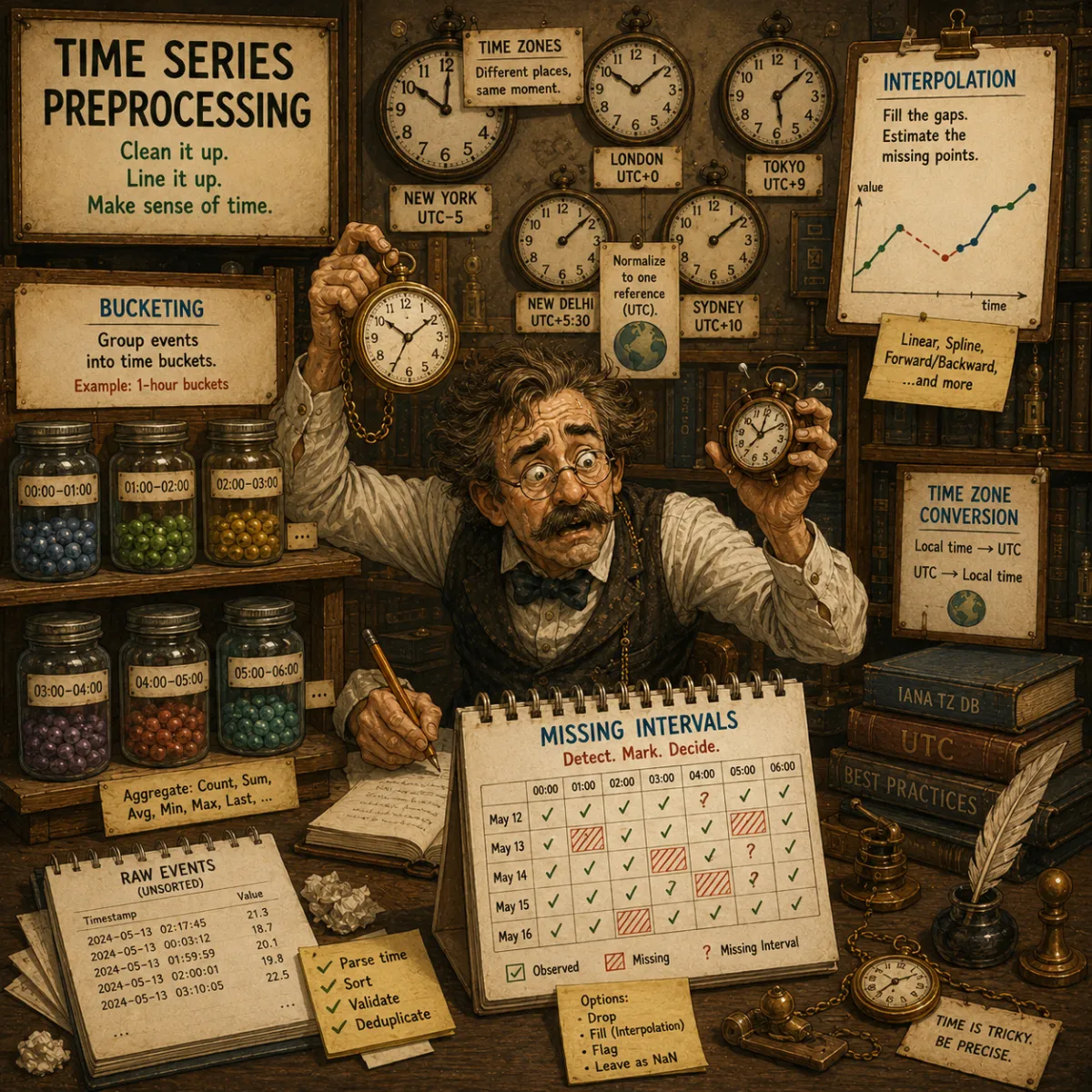
A hands-on explanation of how raw time series data is cleaned, regularized, interpolated, bucketed, and prepared for reliable modeling or visualization.
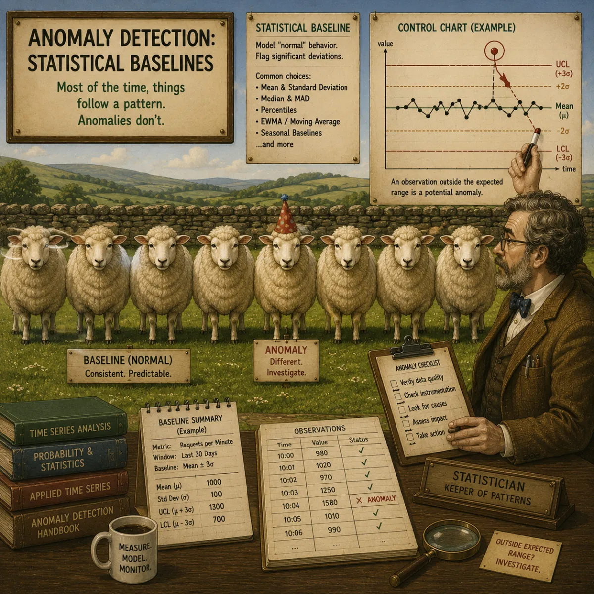
An introduction to statistical baseline methods for time-series anomaly detection: Z-Score, IQR, moving averages, simple ensembles, and evaluation metrics.
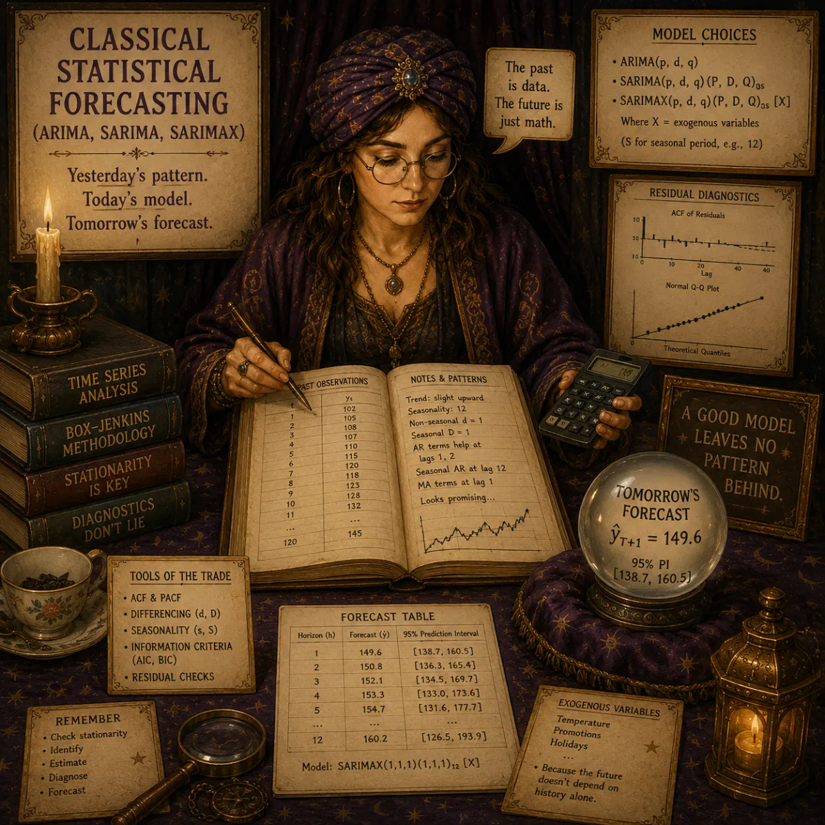
A practical guide to ARIMA, SARIMA, and SARIMAX: how classical statistical forecasting models handle autocorrelation, differencing, seasonality, external regressors, diagnostics, and where they still fit in modern forecasting.
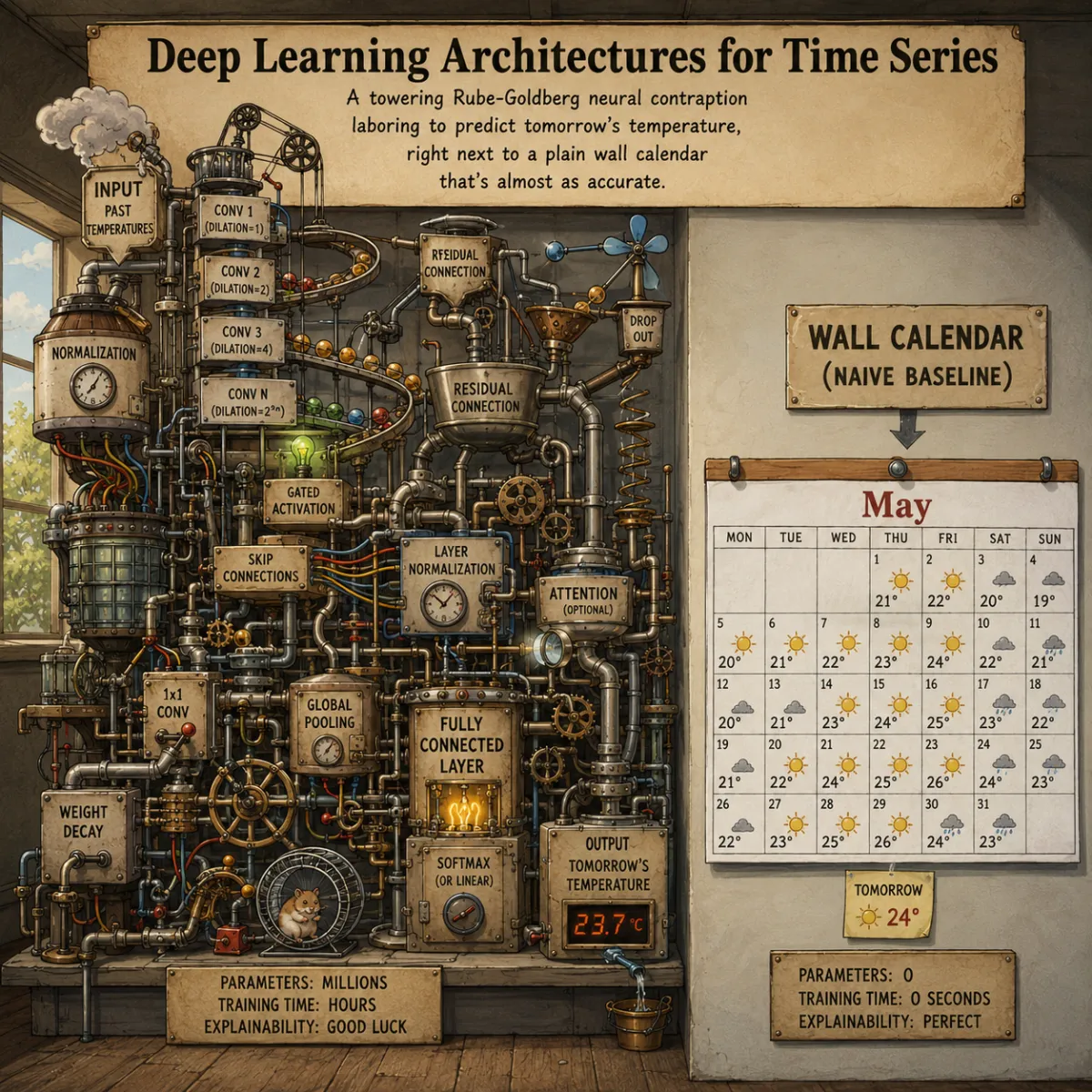
An overview of deep learning architectures for time-series forecasting: LSTM, TCN, DeepAR, N-BEATS, and TFT, with a focus on input shapes, local vs global training, covariates, probabilistic outputs, and practical model selection.
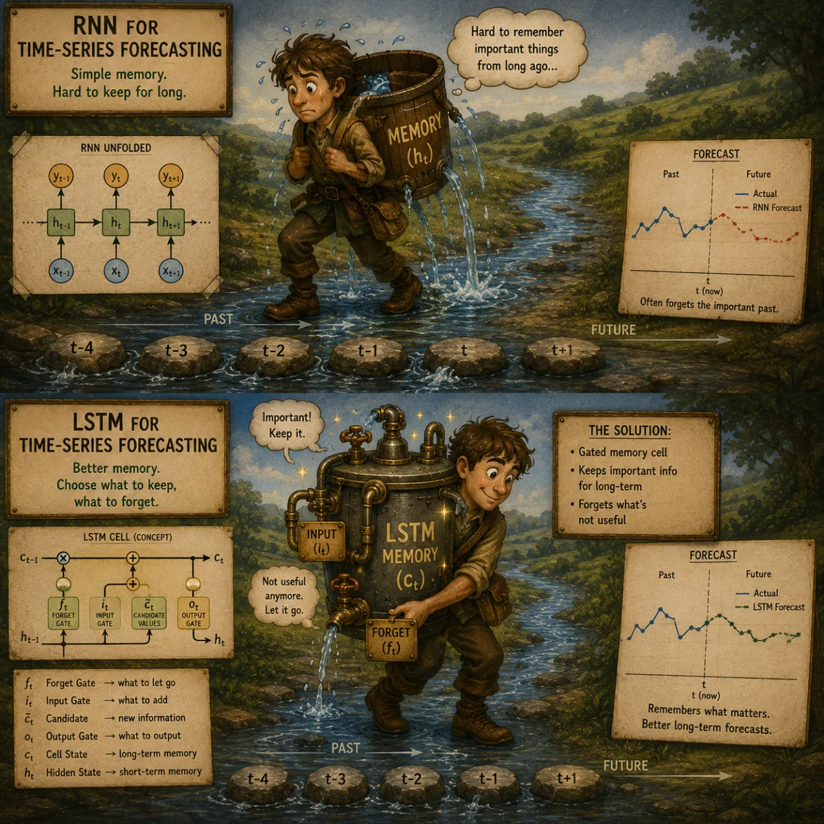
How recurrent networks model sequences: vanilla RNN, the vanishing-gradient problem, the LSTM gating mechanism, cell state, and the practical use of return_sequences in Keras.
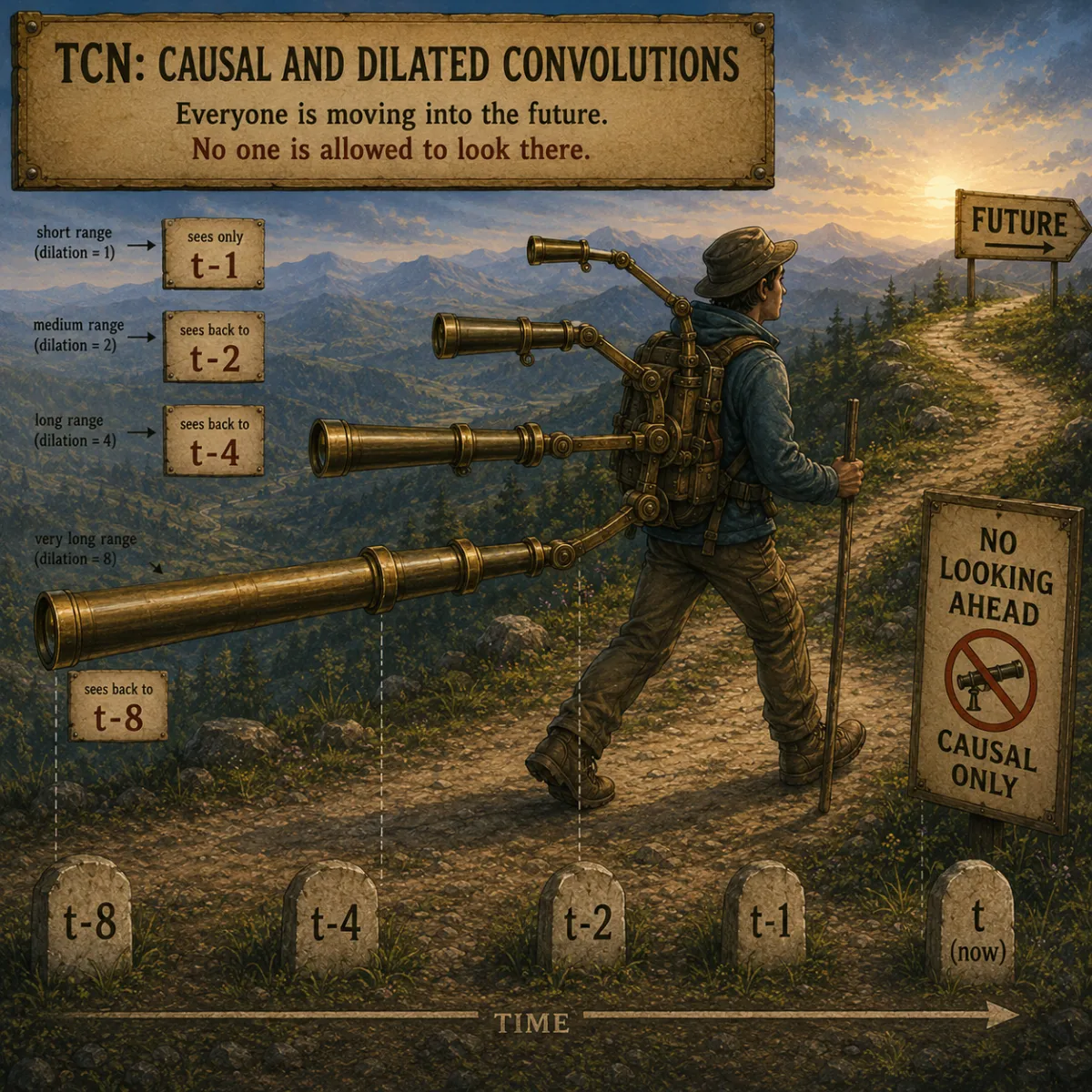
A practical explanation of Temporal Convolutional Networks for time-series forecasting: causal convolutions, dilations, receptive field, residual blocks, optional GLU gating, output heads, and when TCN is useful as a standalone or hybrid forecasting component.
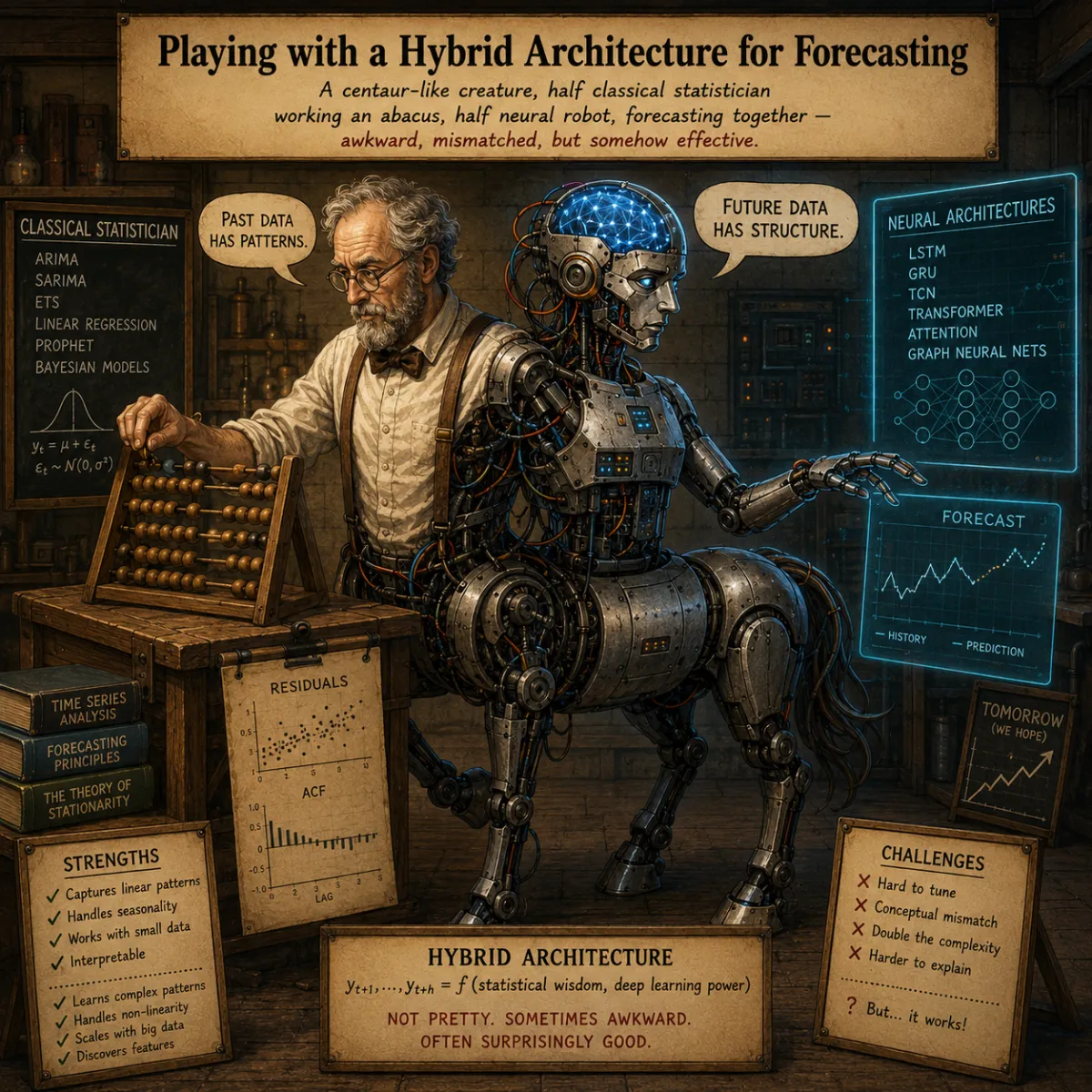
Playing with a hybrid forecasting architecture, assembled out of common neural building blocks: TCN front-end, LSTM recurrence, multi-head attention, TFT-style VSN feature routing with GRN, N-BEATS-style decomposition heads, seasonal and event branches.
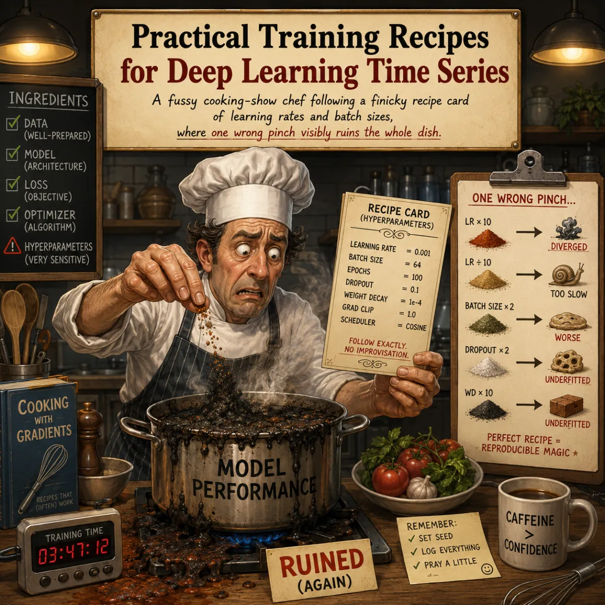
A practical checklist for training deep learning time-series models, covering windowing, initialization, embeddings, regularization, optimizers, learning-rate schedules, loss functions, and the Keras training workflow.
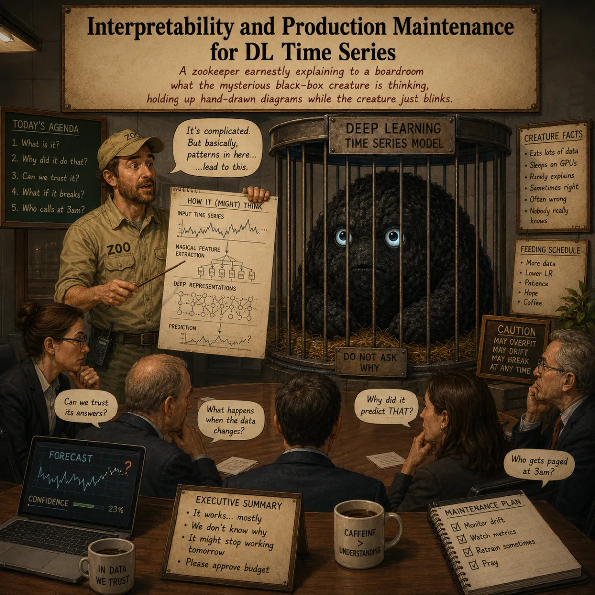
A practical guide to the post-training lifecycle of deep learning forecasters, covering SHAP-based prediction explanations, lightweight recalibration for drift, and the broader production-maintenance roadmap.
Random k-fold CV reshuffles time. On time series that means training on the future to predict the past — and quietly inflating every metric. The correct alternatives are expanding-window and rolling-window CV.
Three components, one additive identity. STL splits a series into trend, seasonality, and residual so you can see what's actually in it before modeling — and the same decomposition idea propagates into modern deep architectures like N-BEATS.
TCN stands for Temporal Convolutional Network — a causal CNN with dilated convolutions that gives sequence models exponential receptive field for the cost of linear depth.
Univariate is one signal over time. Multivariate is many signals over time. The decision between them is about whether the extra signals actually carry information about the target.
ARIMA in three letters: AutoRegression, Integration, Moving Average. SARIMA adds seasonal versions of each. Together they handle the linear, stationary case — which covers a surprising amount of forecasting.
Each interpolation method makes a different assumption about what was happening between known measurements. The right method depends on what the signal actually does between samples, not on what's the default.
TS preprocessing is a pipeline, not a checklist. The order of steps changes the result — scaling before handling missing values is the common trap.
Time series is one entity over time. Panel data is many entities over time. The new dimension — unit-level heterogeneity — is what panel methods exist to handle.