TCN: Causal and Dilated Convolutions for Time Series Forecasting

TCN is the convolutional alternative to recurrent networks for sequence modeling. It is described separately because the building blocks — causal padding, dilations, residual connections, and optional gated activations such as GLU — show up not only in standalone TCN models but also as components of all kinds of custom hybrid forecasting architectures, where TCN often sits in front of LSTM as a parallel feature extractor. This note covers the TCN block itself; the architectures overview places it next to RNN/LSTM, N-BEATS, and TFT.

---

TCN — Temporal Convolutional Network

TCN — Temporal Convolutional Network — an alternative architecture for sequence modeling, popularized as a generic sequence-modeling architecture by Bai, Kolter, and Koltun in 2018, building on earlier ideas such as causal and dilated convolutions (notably from WaveNet). The Bai et al. paper showed that on a wide range of tasks, properly designed convolutional networks can match or beat recurrent ones, including LSTM and GRU.

This is why TCN often appears not only as a standalone model but also as a front-end feature extractor before LSTM or attention: the convolutional block quickly extracts local and medium-range temporal patterns, while the next block handles recurrence or longer-range interactions.

Main idea

Idea: an alternative to RNN via 1D convolutions with causal padding and dilations. Trains efficiently through parallel convolution and gives a large, explicitly controllable receptive field.

The main insight of TCN: to process sequences, it's not necessary to use recurrent connections, which parallelize poorly and suffer from gradient issues. Instead, you can use 1D convolutions (convolution applied to the sequence dimension), but with two important modifications:

• Causal padding — so the model doesn't see the future.
• Dilations — to expand the receptive field.

The result: a network that trains in parallel (all timesteps simultaneously in one forward pass) and suffers far less from vanishing gradients than vanilla RNNs. Unlike LSTM, TCN does not have a theoretically unbounded memory: it only sees as far back as its receptive field allows. This is a strength because the context size is explicit and controllable, but it also means the receptive field has to be designed around the longest lag the task actually needs.

Causal convolution

1. Causal convolution — convolution that doesn't see the future:

Regular conv:   may use both past and future positions around t.
Causal conv:    uses only positions up to t.

In Keras: padding='causal' — adds padding only on the left.

A regular 1D convolution at step t uses values from a window around t — both in the past and in the future. For image processing this is normal, but for time series forecasting it's a catastrophe: the model "peeks" into the future and gets near-perfect accuracy on training — but is unreproducible in production, where the future doesn't yet exist.

Causal convolution solves the problem: the output at step t depends only on inputs from the past (t-k, ..., t), but not from the future. Technically this is achieved through asymmetric padding — adding zero values to the left of the input so that the conv window "looks back". In Keras padding='causal' does this automatically.

There is one important caveat: causal padding only prevents leakage within the convolution window. It does not protect you if the input features themselves contain future information that would not be known at prediction time. Calendar variables (day-of-week, month, holiday flags) are fine — they are known in advance. Future weather observations, future sales, or any feature derived from values past the forecast origin are not, and feeding them in will cheerfully produce a beautiful in-sample forecast that is unreproducible in production.

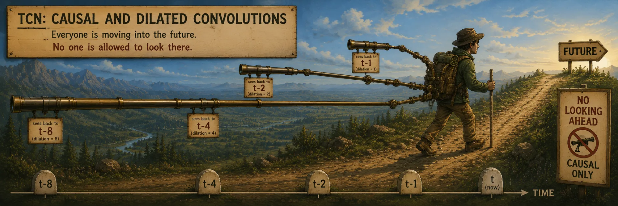
Dilated convolutions

2. Dilated convolutions — larger receptive field with the same kernel size:

Layer 1: dilation=1, sees [t-2, t-1, t]      (kernel_size=3)
Layer 2: dilation=2, sees [t-4, t-2, t]
Layer 3: dilation=4, sees [t-8, t-4, t]
Layer L: dilation=2^(L-1)

These examples describe the positions touched by a single convolutional kernel at that layer. The effective receptive field of the whole stack is larger, because each of those positions already contains information aggregated by previous layers. For a stack with one convolution per dilation level and dilations 1, 2, 4, ..., 2^(L−1), the receptive field is

r = 1 + (k − 1) × (2^L − 1)

For k = 3 and L = 4, this gives a receptive field of 31 input time positions: the current step plus 30 previous steps. The convolutional computation is still parallelizable across time steps, unlike recurrent processing.

If the residual block contains two convolutions with the same dilation (a common variant from the original Bai et al. paper), the convolutional contribution doubles:

r = 1 + 2 × (k − 1) × (2^L − 1)

For k = 3 and L = 4, this gives a receptive field of 61 input time positions (current step plus 60 previous). The point is that the formula depends on how the block is structured, not just on the number of dilation levels — it is worth deriving the receptive field for your specific architecture rather than reading off a single number.

Dilated convolutions — an even more clever trick for extending receptive field without enlarging the kernel. Dilation is the "step" between elements of the convolution kernel.

• With dilation=1 — regular conv: kernel size=3 looks at 3 neighboring timesteps.
• With dilation=2 the kernel looks at every 2nd timestep: [t-4, t-2, t] — same 3 positions, but covering a 5-step window.
• With dilation=4 — 9-step window.

If dilation doubles with each layer (1, 2, 4, 8, ...), the receptive field grows exponentially with the depth of the network. For comparison, LSTM has a theoretically unlimited receptive field, but in practice very long-range dependencies are hard to learn reliably. TCN with dilated convolutions trades the unbounded-but-fragile recurrent memory for a bounded-but-explicit convolutional one, with the benefit of full parallelization.

Building a TCN via a simple loop:

for i in range(tcn_layers):
    dilation = 2**i              # 1, 2, 4, 8, ...
    conv_out = layers.Conv1D(
        filters=tcn_filters * 2,
        kernel_size=tcn_kernel_size,
        dilation_rate=dilation,
        padding="causal",
    )(x)

tcn_layers iterations (usually 4–6), each next one with dilation = 2^i. Keras Conv1D with dilation_rate=dilation does the heavy lifting. padding="causal" ensures the anti-leakage property. filters=tcn_filters * 2 — we specifically double the number of filters for GLU activation, more on which below.

Activation: ReLU and the GLU extension

The original TCN formulation uses causal dilated convolutions, residual connections, dropout/normalization, and a standard nonlinearity such as ReLU. ReLU is a fine default in most cases — fast, simple, well-understood. It can occasionally suffer from "dead neurons" when many activations are stuck at zero, but on convolutional stacks with proper initialization this is rarely a major problem in practice.

In custom hybrid forecasting architectures, it is also common to replace the activation with a gated variant, most often GLU (Gated Linear Unit, Dauphin et al., 2016 — "Language Modeling with Gated Convolutional Networks"). This is not part of the canonical TCN block from Bai et al.; it is a useful extension when we want convolutional feature extraction with LSTM-like gating, often inside the kind of bespoke hybrid forecasting assemblies walked through separately as one example.

conv_out = layers.Lambda(
    lambda t: t[..., :D//2] * tf.sigmoid(t[..., D//2:])
)(conv_out)

The convolution outputs 2D channels (this is why we set filters=tcn_filters * 2 in the loop above), then split in half:

• First half (A) — the "value" component.
• Second half (B) — the "gate".
• Output: A * σ(B) — the sigmoid converts B into values between 0 and 1, which multiplicatively control what part of A passes through.

Why use GLU instead of a plain activation? GLU is not universally better than ReLU; it is roughly twice as expensive in parameters (since the conv has to produce 2D channels) and the gate can saturate. It is useful when we want a learned gate over convolutional features: one half of the channels proposes values, the other half decides how much of those values should pass through. The gradient through the value path stays linear, which avoids tanh/sigmoid-style saturation, and the gate gives the kind of multiplicative control familiar from LSTM. On hybrid architectures that already lean on gating elsewhere it usually fits more naturally than plain ReLU; on a pure TCN baseline ReLU is still the safer default.

Residual connection in TCN

4. Residual connection — the same idea as in ResNet (He et al., 2015):

x_residual = layers.Conv1D(filters=tcn_filters, kernel_size=1, padding="same")(x)
conv_out = layers.Add()([conv_out, x_residual])

A residual connection changes the block from output = F(input) to output = F(input) + input. This gives the gradient a shortcut around the convolutional transformation and makes deep stacks much easier to train. If the number of channels changes inside the block, the input is projected with a 1×1 convolution (Conv1D(kernel_size=1)) so that the residual Add has compatible shapes — that convolution does not look at temporal context, it just linearly transforms channels.

---

A full TCN block

The four pieces above — causal dilated convolution, activation, dropout/normalization, and a residual connection — are usually combined into a single repeatable TCN block. A typical structure looks like this:

input
  → causal dilated Conv1D
  → activation (ReLU or GLU) / dropout / normalization
  → causal dilated Conv1D    (often the same dilation within the block)
  → activation / dropout
  → residual projection (Conv1D kernel_size=1) if channel count changed
  → Add(input, transformed)
output

A TCN model is then a stack of these blocks; the next block typically increases the dilation, in the canonical pattern 1, 2, 4, 8, .... Every block keeps a residual path so gradients can flow regardless of depth, and every block expands the receptive field by its own dilation.

Shape flow

A useful sanity check when designing a TCN forecaster is to track tensor shapes through one block. With D filters per block, kernel size k, and the GLU variant of the activation:

Input:                       (batch, window_size, n_features)
Conv1D(filters=2D, k, ...):  (batch, window_size, 2D)     # 2D channels for GLU
GLU split + gate:            (batch, window_size, D)      # back to D channels
Dropout / LayerNorm:         (batch, window_size, D)
Residual Add:                (batch, window_size, D)      # input projected to D if needed

Two things to keep an eye on: with causal padding the time dimension does not change between layers, which makes the shape arithmetic simple but also means that window_size has to be chosen so that the receptive field actually covers the longest dependency you care about. And with GLU the convolution must produce 2D channels, not D, since half of them become the gate.

---

Choosing the receptive field in practice

A useful rule when designing a TCN forecaster is to size the receptive field around the longest dependency the model should be able to use. The receptive field is bounded and has to be paid for in depth and parameters, so it is worth being explicit about what it needs to cover.

A few worked-out cases for the canonical "one conv per dilation level" form (r = 1 + (k − 1) × (2^L − 1)):

• Hourly data with daily seasonality: the receptive field should cover at least 24 steps. With k = 3, four dilation levels (1, 2, 4, 8) give r = 31 — comfortably enough.
• Daily data with weekly seasonality: at least 7 steps. Even three layers (1, 2, 4) and k = 3 give r = 15.
• Hourly data with weekly seasonality: at least 168 steps. With k = 3, you need 2^L − 1 ≥ 84, i.e. L ≥ 7 (which gives r = 255). At that point the model is starting to get deep, but still trains fast.
• Daily data with yearly seasonality: the receptive field should cover roughly 365 daily positions. The same arithmetic gives L ≥ 8 (r = 511). Possible, but at this scale a plain TCN is starting to be inefficient — explicit calendar features, Fourier seasonality terms, an attention layer, or a different architecture entirely will usually serve better than just stacking more dilated convs.

The general guideline: if your task needs a weekly pattern in hourly data, 31 hours of receptive field is not enough; you either need a deeper TCN that actually covers 168+ hours, or explicit calendar features that let a smaller TCN learn the pattern indirectly. Either approach is fine, but they have to be a deliberate decision rather than an oversight.

---

Output heads for forecasting

A TCN block (or a stack of them) is only the encoder — it produces a sequence of feature vectors (batch, window_size, D). To turn that into a forecast you need a head, and there are a few common patterns:

• Last-step + Dense head. Take the encoder output at the last time step and predict the whole horizon: Dense(horizon)(tcn_out[:, -1, :]). This is the most common pattern for direct multi-output forecasting on top of TCN.
• TimeDistributed head. Keep the full sequence and apply a small Dense network to each time step independently. Useful if you want a per-step forecast (e.g. one prediction per past step, or sequence labeling).
• Pool / flatten + Dense. Pool the encoder output across time (global average / max pooling) or flatten it, then predict the horizon. This loses sharp temporal localization but compresses well.
• TCN as a feature extractor inside a hybrid. Pass the TCN output into LSTM, attention, or a TFT-style decoder. This is what the bespoke hybrid assembly walked through separately does, using TCN as the front-end before recurrence.

Which head you pick is a separate design choice from the TCN encoder itself. The encoder gives you a clean per-step representation; the head decides how that representation becomes a horizon forecast.

---

Common mistakes

A short list of TCN-specific gotchas that show up in production code:

1. Setting padding="same" instead of padding="causal" and accidentally leaking future target values into the convolution window. Symptom: training loss looks suspiciously good and validation falls apart.
2. Increasing the lookback window without checking the receptive field. A 365-step input window does not magically give the model a 365-step receptive field; if the dilations only cover 31 positions, the extra inputs are wasted (or worse, only the most recent slice is actually used).
3. Assuming a TCN can learn yearly seasonality just because the input window contains a year of data. Without enough dilation depth or explicit seasonal features, the model literally cannot reach back that far.
4. Using GLU but forgetting to double the number of convolution filters before splitting channels. Without filters = 2D, the channel split has nothing to split, and shapes break in confusing ways further down the network.
5. Treating causal padding as protection against feature leakage. Causal padding only fixes leakage within the convolution window; it does not protect you from input features that already encode the future (next week's promo flag fed in as if it were observed today).

---

When to use TCN, and when to be careful

TCN is the natural choice when:

• you need a long lookback window and training speed matters — convolutional stacks parallelize across time in a way that recurrent networks cannot;
• the relevant history length can be covered by a finite, explicit receptive field that you are willing to size up front;
• you want a convolutional feature extractor in front of an LSTM, attention layer, or other sequence model — the hybrid pattern.

It is worth being careful when:

• the dependencies you need extend further back than your receptive field, and adding more layers or wider kernels makes the model too expensive — beyond some point an LSTM, an attention model, or a foundation model is a better fit;
• the data has irregular timestamps — convolution implicitly assumes a regular grid, so irregular series typically need to be aligned to one first (the time-series preprocessing note covers this);
• some of the input features would only be known after the forecast origin — causal padding does not protect you from feature-level leakage, only from kernel-window leakage;
• the forecasting task needs flexible memory beyond a fixed window (e.g. very long-tail seasonal effects), in which case a model with explicitly long-context attention or a foundation model is usually the right answer.

In other words: TCN is a strong and fast convolutional encoder for sequences, but it is bounded by its receptive field, and that bound has to be designed deliberately rather than hoped for.