Chapter 1 of 4
Data Storage Formats
Created Apr 28, 2026 Updated May 4, 2026
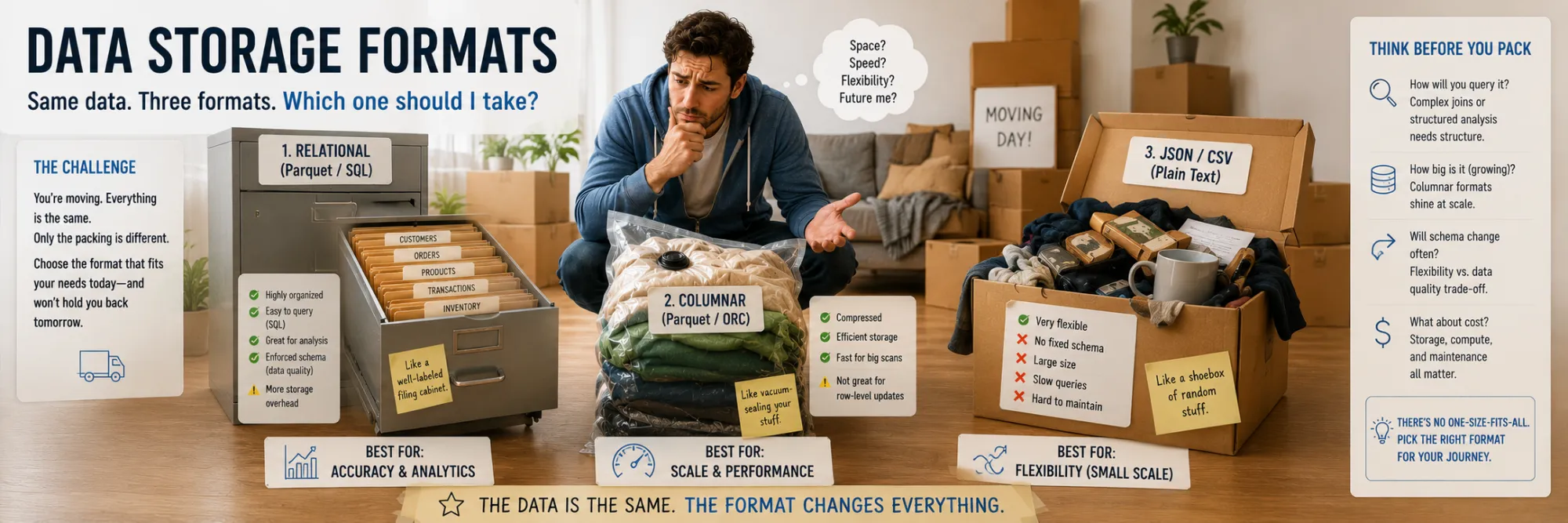
A storage format is a convention for how a sequence of bytes on disk turns into meaningful records: rows, columns, nested objects. The choice of format determines three important characteristics: file size on disk, read and write speed, and ease of integration with other tools. No single format wins on all three metrics simultaneously — and that is why several formats usually coexist in real systems, each serving its own role.
In this chapter we examine the three most widespread formats in order from the simplest to the most optimized: CSV as the textual tabular standard, JSON as the textual format for nested structures, and Parquet as the binary columnar format for analytics.
CSV
CSV (Comma-Separated Values) is the oldest and at the same time still the most widespread textual format for tabular data. Despite all of its drawbacks and the appearance of more efficient alternatives, it remains the de facto standard for exchanging data with the business: Excel opens CSV, Google Sheets imports CSV, and any BI tool can work with it.
The format appeared back in the 1970s, long before any modern structured data formats existed. The first formal specification — RFC 4180 — was only published in 2005, which on its own says a lot about the chaotic nature of its use: for decades different tools implemented CSV slightly differently, and these inconsistencies still surface in edge cases.
Strengths:
- Universality. Any tool in the world — from Excel to SAP, from Postgres
COPYto a plaincat file.csvin the terminal — can work with it. - Human-readability. You can open the file in a text editor and see a table.
- Simplicity. A parser can be written in half an hour (although a correct parser that properly handles escaping is rather more involved).
This universality makes CSV the ideal "lowest common denominator" for exchange between systems that don't want to agree on more complex formats.
Weaknesses:
- No schema. All values are strings; types have to be guessed (type inference). The number
"007"may end up as the string"007"or as the number7, depending on what the parser decides. - Escaping hell. If a value contains a comma, a quote, or a line break, it has to be escaped correctly, and different tools do this in different ways.
- Size and parse speed. On analytical workloads, CSV can easily be several times larger and much slower to parse than Parquet, especially when only a subset of columns is needed. Exact ratios depend on the data, the query, and the engine, but the gap is large enough to matter for any non-trivial pipeline.
- No built-in compression. You can wrap it in gzip, but then you lose the ability to do random access — you have to decompress the whole file at once.
Python's standard library has the csv module, which correctly handles most edge cases: escaping, different quote styles, dialects (Excel vs Unix). This is enough for typical tasks on small volumes. For large datasets it is slow, because it works row-by-row through the Python interpreter.
For large CSV files there are performant alternatives. polars.read_csv(streaming=True) reads the file as a stream without loading everything into memory, with multithreaded parsing in Rust. duckdb.read_csv_auto() performs schema inference and lets you run SQL directly against CSV without an explicit load into a table. Both approaches deliver several-times speedups compared to stdlib csv and pandas.read_csv.
The typical niche for CSV today is the final export for business users. Inside the pipeline data usually lives in more efficient formats (Parquet), and is converted to CSV only at the boundary, when the result needs to be handed off to an analyst who will open the file in Excel or import it into Tableau / Power BI. This is a stable pattern: fast internal formats for processing, CSV — for interaction with human-facing tools.
Write a DataFrame to CSV and read it back. What happens to the column types?
import pandas as pd import iodf = pd.DataFrame({ "id": pd.array([1, 2, 3], dtype="int32"), "score": [0.95, 0.87, 0.91], "date": pd.to_datetime(["2024-01-01", "2024-01-02", "2024-01-03"]), "status": pd.array(["active", "pending", "active"], dtype="string"), })
print("Before CSV roundtrip:") print(df.dtypes) print()
buf = io.StringIO() df.to_csv(buf, index=False) buf.seek(0) df2 = pd.read_csv(buf)
print("After CSV roundtrip:") print(df2.dtypes)
JSON
JSON (JavaScript Object Notation) is the most widespread data interchange format in modern web development. Invented by Douglas Crockford in 2001 as a subset of JavaScript object syntax, it was standardized in RFC 8259. Practically any HTTP API today returns JSON, any config file (other than YAML/TOML) is JSON, any exchange between frontend and backend is JSON.
JSON's main advantage is universality and simplicity. Every programming language has high-quality JSON parsers, the format is easy to read for humans, and the structure naturally expresses nested objects and arrays. Compared to XML, which dominated before it, JSON is dramatically more concise: less boilerplate, no namespaces, and no complex schema by default.
Data types. JSON is intentionally minimalist: only object (dictionary), array (list), string, number, boolean, and null are supported. There are no dates, no binary data, and no distinction between integer and float (in JSON 42 and 42.0 are the same number type). This creates several practical problems:
- Dates are usually serialized as ISO strings of the form
"2024-04-22T10:30:00Z"and parsed as dates on the client side. - Binary data is transmitted as base64 strings, which inflates the size by 33%.
- Large integers (int64) lose precision when parsed in JavaScript, because JS numbers are float64 with a precision limit of about
2^53.
Python's standard library has the json module. It is convenient and fast enough for most tasks (CPython ships C-accelerated decoders / encoders by default), but on hot paths processing millions of JSON objects it can become a bottleneck. For high loads, alternatives are used:
- orjson (written in Rust) — about 5 times faster than the stdlib and correctly handles
datetimeandUUIDwithout a custom encoder. - ujson (C) — faster than the stdlib, but less full-featured.
For FastAPI and other modern frameworks, orjson is usually chosen by default when serialization performance matters.
When JSON is the right choice:
- REST API requests and responses, where the data structure is heterogeneous and nested, and the endpoints of the conversation are separate services.
- Configuration files with simple structure (but if comments are needed, YAML or TOML is better).
- Nested structures of arbitrary depth.
- Interaction with JavaScript, where JSON is natively parsed into an object with a single
JSON.parse()call.
When JSON is a poor choice:
- Large tabular data. Parquet is several times more efficient in size and read speed.
- Streaming. A regular JSON document is not naturally record-streamable: if the file is one large array or object, the reader usually has to understand the document structure as a whole. Streaming JSON parsers exist (
ijson, SAX-style approaches), but they push the structural complexity onto the consumer. JSON Lines (.jsonl) solves this by placing one complete JSON object per line. Because each line is independently valid JSON, a reader can process records one at a time without loading the full file — memory usage stays flat regardless of file size. In practice you will see JSONL wherever streaming matters: fine-tuning datasets for LLMs (OpenAI and HuggingFace both use it as their standard format), log aggregation pipelines, and any situation where a producer appends records incrementally. - Binary data. Base64 encoding is inefficient; if you have to ship a lot of binaries, it is better to look toward MessagePack, Protobuf, or Avro.
In practice JSON is especially convenient in two typical scenarios. The first is storing structured data generated by LLMs: modern language models natively emit JSON, and no extra conversion is required. The second is exchange between frontend and backend in web applications: Pydantic models (or their equivalents in other ecosystems) are automatically serialized to JSON when returned from a handler and parsed from JSON when receiving a request, so the developer never sees the raw bytes at all.
Parquet
Parquet is a columnar binary data storage format, developed by Twitter and Cloudera in 2013 and donated to the Apache Foundation. It was originally created for the Hadoop ecosystem, but has since become the de facto standard for data lakes and analytical processing. The format is binary and self-describing — the schema is embedded into the file itself, no separate CREATE TABLE or external catalog is needed.
File structure
A Parquet file has a hierarchical structure. As an example, consider a typical events table with columns user_id, timestamp, amount:
Parquet File
├── Row Group 1 (logically — a "batch" of rows, ~128 MB by default)
│   ├── Column Chunk: user_id    ← all user_id values of this row group in sequence
│   │   └── Pages (compressed chunks, Snappy/Gzip/Zstd)
│   ├── Column Chunk: timestamp
│   └── Column Chunk: amount
├── Row Group 2
├── ...
└── Footer
    ├── Schema
    ├── Row Group metadata (min/max per column)
    └── Statistics
At the top level the file is divided into row groups — logical batches of rows, around 128 MB each by default. Inside a row group the data is physically laid out by column: first all the values of the user_id column from this batch in sequence (this is called a column chunk), then all the values of timestamp, then amount. Each column chunk is split into pages — compressed blocks to which Snappy (fast compression with an acceptable ratio), Gzip (legacy, slower than Snappy), or Zstd (modern, best ratio at good speed) is applied. At the end of the file is the footer with metadata: the schema, the boundaries of row groups, and min/max statistics for each column in each row group.
Why Parquet is fast
The first and third optimizations below come from the columnar layout itself; the second is a Parquet file format feature built on top of it.
The advantage of a columnar format shows up especially clearly on analytical queries. Imagine a table with 50 columns and a million rows and a query SELECT AVG(amount) FROM events WHERE user_id = 'abc'. A row-oriented format such as CSV or JSON is forced to read all 50 columns for all million rows from disk, parse them, and then discard the 48 unneeded columns. A huge amount of time is spent at the I/O stage on data that is never used. Parquet reads only two columns — user_id and amount — skipping the other 48. The I/O saving is on the order of 96%, and that is the simplest advantage of the columnar approach.
The next level of optimization is predicate pushdown. Since the footer stores min/max for each column in each row group, for a filter like WHERE user_id = 'abc' the query engine can first read only the footer (kilobytes), look at the statistics, and decide: this row group definitely does not contain the needed data — there is no need to open it at all. The algorithm looks like this:
- Read only the footer (kilobytes).
- Look at the min/max
user_idof each row group. - Skip row groups where
'abc'does not fall in the range. - Read only the remaining row groups.
If the data is sorted by the filtered column, this skips up to 99% of the file.
The third source of speed is compression. Because a column stores values of the same type — often with many repeats — columnar data compresses far better than rows do. Columns with repeating values (timestamps, enums, identifiers) can shrink by tens or hundreds of times thanks to two techniques. Dictionary encoding replaces repeating string values with short integer indices and stores the dictionary separately. Run-length encoding (RLE) represents a sequence of identical values as a pair "value × number of repetitions". In CSV the string "user_42,user_42,user_42,user_42" takes 32 bytes; in Parquet this turns into user_42 × 4 — literally a few bytes.
Typing
Typing in Parquet is rich: int32 and int64, float and double, string and binary, timestamp and date, decimal with arbitrary precision, and also nested structures — list, struct, and map. The latter is important for JSON-like data, which you don't have to flatten into flat tables.
Partitioning
Partitioning is usually implemented at the file system level via a path convention:
data/
  year=2026/
    month=04/
      day=22/
        part-0001.parquet
        part-0002.parquet
The query engine sees the filter WHERE year=2026 AND month=04 and immediately understands that only one folder needs to be opened — the others are not even scanned. This is partition pruning, and it works even before any Parquet files start being read at all — that is, it is cheaper than predicate pushdown.
Alternatives
The main alternatives to Parquet are:
- ORC (Optimized Row Columnar) — developed by the Hive community, functionally very close to Parquet, but less popular outside the Hadoop stack.
- Avro — row-based, better suited for streaming and messaging than for analytics.
- Delta Lake and Apache Iceberg — modern table formats, both using Parquet as the storage layer and adding ACID metadata, time travel, and schema evolution on top.
Parquet stores schema in the file and supports typed data well, but schema evolution across many files in a dataset (renaming, dropping, or relaxing types over time) is usually managed by the query engine or a higher-level table format such as Delta Lake or Iceberg. The Parquet file itself only describes its own schema.
In most modern analytical pipelines, Parquet is the default internal storage format rather than an exotic optimisation: it saves I/O, is natively read by all the major engines (Spark, Trino, DuckDB, Polars, pandas via PyArrow), and integrates cleanly with table-format layers when transactional or evolution guarantees are needed.
Same DataFrame, same roundtrip — but through Parquet. Compare the types with what CSV produced above.
import pandas as pd import pyarrow as pa import pyarrow.parquet as pq import iodf = pd.DataFrame({ "id": pd.array([1, 2, 3], dtype="int32"), "score": [0.95, 0.87, 0.91], "date": pd.to_datetime(["2024-01-01", "2024-01-02", "2024-01-03"]), "status": pd.array(["active", "pending", "active"], dtype="string"), })
print("Before Parquet roundtrip:") print(df.dtypes) print()
buf = io.BytesIO() df.to_parquet(buf, index=False) buf.seek(0) df2 = pd.read_parquet(buf)
print("After Parquet roundtrip:") print(df2.dtypes)
Comparison
No single format wins on every dimension. The table below summarises where each one fits.
| CSV | JSON | Parquet | |
|---|---|---|---|
| Encoding | text | text | binary |
| Schema | none (inferred) | none (inferred) | embedded in file |
| Types | strings only | string, number, bool, null | rich: int32/64, float, timestamp, decimal, nested |
| Nested data | no | yes | yes (list, struct, map) |
| Human-readable | yes | yes | no |
| Compression | none built-in | none built-in | built-in (Snappy / Zstd / Gzip) |
| Read speed | slow | slow | fast |
| Streaming | line-by-line | JSONL only | row groups |
| Efficient partial reads | no | no | yes (column pruning, row-group skipping) |
| Typical role | export to business tools | APIs, configs, LLM data | internal pipeline storage, analytics |
How to choose
A short decision rule that follows from the table:
- CSV when the file is meant for humans or business tools — Excel, Google Sheets, Tableau, Power BI, ad-hoc handover to an analyst.
- JSON when the data is nested, exchanged through APIs, or produced and consumed by web services. Configs, REST payloads, LLM-generated structured outputs.
- JSONL when records arrive incrementally or need to be streamed: log pipelines, LLM fine-tuning datasets, append-only event collection.
- Parquet when the data is tabular, large, analytical, and read repeatedly by query engines. The default for internal pipeline storage.
- Delta Lake or Iceberg when you need table-level guarantees on top of Parquet: transactions, time travel, schema evolution across many files, deletes and updates with consistency.