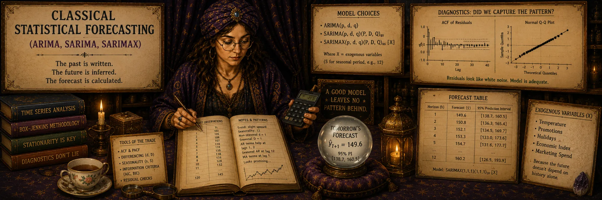
Classical Statistical Forecasting: ARIMA, SARIMA, and SARIMAX

The classical statistical tradition of time series forecasting is significantly older than modern machine learning. Long before neural networks and boosting, statisticians developed a series of models that for decades were the workhorse for forecasting in economics, finance, and engineering. Even today, in the era of foundation models, these models remain important — as a baseline, as an interpretable instrument for regulated industries, as a way of working with small data.

At the center of this tradition is the ARIMA family and its extensions — SARIMA (accounting for seasonality) and SARIMAX (adding external regressors). The sections below cover their structure, assumptions, practical methodology for parameter selection, and edge cases where they are poorly suited.

---

ARIMA: the basic model

ARIMA is the central model of the Box–Jenkins tradition. It combines three ideas — autoregression, differencing, and moving-average errors — into one compact framework for modeling a single time series. The name itself is just an abbreviation of those pieces: AutoRegressive Integrated Moving Average.

ARIMA(p, d, q) — AutoRegressive Integrated Moving Average.

The model is parameterized by three non-negative integers (p, d, q), each controlling the complexity of one of the three components. The Box–Jenkins methodology (1976) gave practitioners a repeatable procedure for choosing a configuration (p, d, q) for a specific series — the turn from "art" to "method" was the contribution that really propelled ARIMA into mainstream use.

---

The three components of ARIMA

ARIMA decomposes time series dynamics into three separate mathematical components. Each component solves its own task, and together they provide a flexible framework for a broad class of series.

AR(p) — AutoRegressive

The dependence of the current value on past values:

y_t = c + φ₁ y_{t-1} + φ₂ y_{t-2} + ... + φ_p y_{t-p} + ε_t

where p is the order of AR (how many lags we use), φ are the coefficients.

The AR (AutoRegressive) component models the linear dependence of the current value on lags. Formula: y_t is a linear combination of p previous values y_{t-1}, ..., y_{t-p} plus a random error ε_t. The coefficients φ_i are learned from the data.

p is the order of the AR component, indicating how many past values to use. Intuitively: if p = 1, the current value depends only on the immediately preceding one. For daily data, a lag like p = 7 can pick up a dependence on the same day of the previous week, but regular weekly seasonality is usually modeled more explicitly via SARIMA with seasonal period s = 7 — that expresses the weekly pattern through dedicated seasonal structure, instead of forcing the non-seasonal AR part to carry the whole weekly effect, and keeps the modeler honest about why the lag matters. AR(p) is a fundamental building block of classical time-series theory.

I(d) — Integrated (differencing)

Differencing to ensure stationarity:

d=0: original
d=1: y_t - y_{t-1}           (first difference — removes a linear trend)
d=2: (y_t - y_{t-1}) - (y_{t-1} - y_{t-2})   (second — removes a quadratic trend)

In the standard ARIMA formulation, the series after differencing is expected to behave as stationary — with a roughly constant mean, variance, and autocorrelation structure over time (more precisely, weak stationarity, as discussed in the time-series-data note). Real-world series are usually not stationary in their raw form (trend, seasonality, changing variance), and differencing is the standard way of bringing the modeled process closer to that assumption.

In simple polynomial-trend cases the picture is clean: the first difference (d = 1) — subtracting the previous value from the current — removes a linear trend, and the second difference (d = 2) — differences of differences — removes a quadratic one. In real data the trend is rarely a clean polynomial, so differencing should be thought of as a practical tool that reduces trend and brings the series closer to stationary, rather than as a universal trend-removal guarantee. Smoothly curved trends may benefit from a variance-stabilizing transformation (log, Box–Cox) before differencing; piecewise trends or regime changes are a different problem altogether and typically call for change-point handling, intervention variables or a different modeling approach, not for cranking d higher.

After training ARIMA on a differenced series, the forecasts are inverted back to the original scale. d = 0 means that differencing is not needed — the series is already stationary.

MA(q) — Moving Average

Dependence on past errors (not values):

y_t = c + ε_t + θ₁ ε_{t-1} + θ₂ ε_{t-2} + ... + θ_q ε_{t-q}

The MA (Moving Average) component — with a confusing name! It has nothing to do with a simple "average over a period". In reality it models the linear dependence of the current value on past errors — residuals from previous predictions.

Formula: y_t is the sum of the current random error ε_t plus weighted past errors. The idea: shocks to the system have lingering effects. If yesterday's forecast underestimated the actual value, today's value is still partially affected by that discrepancy.

q is the order of the MA component, how many past errors influence the current value.

---

The full ARIMA(p, d, q) formula

Combining all three components:

Δ^d y_t = c + Σ φ_i Δ^d y_{t-i} + ε_t + Σ θ_j ε_{t-j}

The full ARIMA applies d differences to the original series (notation Δ^d), then models the differenced series as a combination of AR(p) + MA(q).

Typical choices: ARIMA(1, 1, 1) — a simple "trend + one lag + one error" model. ARIMA(2, 1, 2) — richer. Higher orders are rarely needed in practice — this is usually a sign of overfitting.

---

How to choose the parameters p, d, q

The choice of the three parameters is a critical step in the ARIMA methodology.

• d is determined via the ADF test (Augmented Dickey–Fuller) for stationarity: increase d until the series becomes stationary.
• p, q — via ACF / PACF plots (autocorrelation, partial autocorrelation functions) or by minimizing AIC/BIC.
• auto_arima (from the pmdarima library) — automatic grid search.

Determining d via the ADF test

The ADF test (Augmented Dickey–Fuller) is a statistical test built around the unit-root null hypothesis: the series is non-stationary (has a unit root). If the p-value is less than 0.05, the unit-root hypothesis is rejected, and the series is treated as stationary for modeling purposes. Strictly speaking the test does not "prove" stationarity — it gives grounds to reject the unit-root assumption — but in practice the rejection is what licenses moving on to ARIMA fitting.

Algorithm: start with d = 0, run ADF. If the series is non-stationary, try d = 1, repeat. Continue differencing until ADF shows stationarity. Usually d = 0, 1 or 2 is sufficient; higher orders are a sign that the series is somehow unusual, and it is worth thinking about transformations (logarithm, Box-Cox) before increasing d.

Determining p and q via ACF/PACF

ACF (AutoCorrelation Function) shows the correlation of the series with its lags (at lag 1, 2, 3, ...). PACF (Partial AutoCorrelation Function) is similar, but with control for intermediate lags.

Theoretical patterns:

• A pure AR(p) has a sharp PACF cutoff at lag p and gradual ACF decay.
• A pure MA(q) — the opposite pattern: a sharp ACF cutoff at lag q, gradual PACF decay.
• Mixed ARMA models — more complex patterns, hard to interpret manually.

The modern automatic approach

The modern way is auto_arima (the pmdarima library), which automates the selection through grid search, minimizing the information criteria AIC (Akaike Information Criterion) or BIC (Bayesian Information Criterion). It substantially reduces the need for manual ACF/PACF inspection and gives a reproducible process. It does not, however, replace diagnostics: automatic selection can pick a model that is statistically convenient (low AIC/BIC, well-fitted in-sample) but practically unreliable — the residuals can still carry structure, the chosen orders can be too high to generalize, and out-of-sample forecasts can drift even when in-sample diagnostics look clean. Treat auto_arima as a strong starting point that still has to be validated, not as the final answer.

A minimal usage looks like this:

from pmdarima import auto_arima

model = auto_arima(
    y,
    seasonal=True,
    m=12,                       # seasonal period (12 for monthly + yearly seasonality)
    information_criterion="aic",
    trace=True,
    suppress_warnings=True,
)

forecast = model.predict(n_periods=12)

The same API supports exogenous regressors via the X argument and switches to SARIMAX-style estimation in that case. There is one practical detail that catches people repeatedly: when exogenous regressors are used in training, their future values must also be supplied at prediction time — model.predict(n_periods=12, X=X_future). Those future values either need to be known in advance (calendar features, holiday indicators, planned promotions) or forecasted separately by another model (weather, prices, marketing spend); otherwise SARIMAX cannot produce a valid future forecast. After fitting, the residuals from model.resid() should be checked for remaining autocorrelation (Ljung–Box test) before the model is trusted.

---

SARIMA: adding seasonality

Plain ARIMA is not designed to represent regular seasonality explicitly — the periodic patterns that repeat with a fixed period (daily routine, weekly cycle, yearly). It can pick up some seasonal effects through high-order non-seasonal lags, but the dedicated extension for the job is SARIMA (Seasonal ARIMA).

SARIMA(p, d, q)(P, D, Q, s) — adds seasonal components:

• Capital letters (P, D, Q) — seasonal AR, seasonal I, seasonal MA.
• s — period (12 for monthly data with yearly seasonality, 7 for daily with weekly).

SARIMA(1, 1, 1)(1, 1, 1, 12):
  non-seasonal AR = 1, I = 1, MA = 1;
  seasonal — the same, period 12.

Seasonal components work the same way as non-seasonal, but at lags equal to the periods. For example, SAR(1) with s = 12 means that the current value depends on the value 12 steps (months) ago — this captures the effect of "last January".

s = 12 — for monthly data with yearly seasonality. s = 7 — for daily data with weekly seasonality. s = 24 — for hourly data with daily seasonality.

---

SARIMAX: external regressors

SARIMAX — SARIMA + eXogenous variables. Adds external regressors to the model:

y_t = β × X_t + ARIMA-part

A linear combination of external features X_t is added to the ARIMA model — holiday indicators, competitor prices, weather, advertising activities.

This makes SARIMAX a bridge between pure time series models and regression: you can simultaneously work with both seasonal dependencies and external drivers. But SARIMAX remains a linear model — complex non-linear interactions between exogenous features are not captured.

A short concrete example to anchor the three models against each other. Suppose we have monthly sales data for a single product:

• ARIMA can model the local momentum and short-term shocks — sales this month depend on the last few months and on the noise that hit them.
• SARIMA additionally learns that every December behaves systematically differently from an average month — a seasonal AR/MA component picks up the yearly cycle without us writing it down by hand.
• SARIMAX can include known external information: a holiday flag, a marketing-spend column, an indicator for a price promotion. The catch is that these enter the model as a mostly linear effect; "spend $1 more on ads, get $k more sales" rather than the saturating, threshold-style relationships that real campaigns usually have.

Reading from ARIMA to SARIMAX is a steady accumulation of structure: more dynamics, more seasonality, more external context — but always within the linear framework of the ARIMA family.

---

ARIMA assumptions

ARIMA produces reliable inference when a handful of statistical assumptions are reasonably met. The important thing is not to treat them as a checklist that returns pass/fail. In practice they tell us what kind of trust we can place in the model: point forecasts may still be useful when the residuals are not perfectly normal, but the prediction intervals around those forecasts become questionable; leftover autocorrelation, on the other hand, is a much stronger sign that the model has missed real temporal structure and needs to be reconsidered. With that framing, the standard list of assumptions is:

• Linearity — the modeled relationships are linear.
• Stationarity — after differencing the series should look stationary.
• Residuals close to white noise — model errors should have no remaining autocorrelation and approximately zero mean.
• Approximate normality of residuals — needed mainly for inference and prediction intervals, less so for point forecasts.
• Homoscedasticity — the variance of the errors is stable over time.

Linearity. The relationships in the standard ARIMA formulation are linear — non-linear patterns (quadratic growth, sigmoidal saturation) are not captured directly. For strongly non-linear series, other methods are usually needed.

Stationarity. The series should look stationary after differencing. If even after d = 2 it is clearly not, that is a sign to step out of the ARIMA frame: try a transformation (log, Box–Cox) or pick a different model entirely, rather than pushing d higher.

Residuals. A well-fitting ARIMA model leaves residuals that behave like white noise: no remaining autocorrelation, mean approximately zero. This is the assumption that really matters for the fit — leftover autocorrelation in the residuals means the model has not captured all the temporal structure, and a richer (p, q) is usually warranted. Approximate normality of the residuals is a separate, weaker requirement: it is what makes confidence intervals, prediction intervals and significance tests meaningful, so it matters most when you actually rely on those quantities. Useful point forecasts can come out of a model whose residuals are not perfectly normal — but the uncertainty around those forecasts will be miscalibrated.

Homoscedasticity. The variance of the errors is stable over time. If the variance grows (financial series often show volatility clustering), this assumption is violated — for such cases GARCH or stochastic-volatility models are more appropriate.

Diagnostic tests

After training ARIMA, the assumptions are verified by diagnostic tests:

• Ljung-Box test — null hypothesis: residuals have no autocorrelation. If p-value < 0.05, unexplained structure remains in the residuals — the model has not captured all patterns, it is worth trying a more complex one (higher p, q).
• Jarque-Bera test — null hypothesis: residuals are normally distributed. Important for inference (confidence intervals, statistical significance). Non-normal residuals still allow point forecasts to be made, but undermine uncertainty quantification.

---

When to use ARIMA

ARIMA tends to work very well in a few specific situations:

• Stable univariate series with autocorrelation and trend — this is ARIMA's native territory, with decades of proven track record. SARIMA extends the same machinery to series with regular seasonality (weekly, yearly, daily-cycle).
• No complex external regressors — ARIMA handles pure temporal dynamics elegantly; complex exogenous interactions are usually better captured by ML methods.
• Interpretability is critical — in regulated industries (healthcare, finance) every coefficient typically has to be explained, and ARIMA provides that out of the box.
• Little data — ARIMA can produce useful forecasts on a few hundred observations, where most ML methods would struggle. For a new product with a year of history, ARIMA is often the only viable choice.

When ARIMA is a poor choice

The flip side:

• Non-linear dynamics — ARIMA is purely linear, cannot capture saturation curves, threshold effects.
• Many exogenous regressors — SARIMAX supports them, but quickly becomes unwieldy beyond a few; ML handles hundreds of features.
• Many parallel series — ARIMA needs to be fit separately for each series; 1000 products = 1000 models, each requiring tuning and maintenance. This is the panel-forecasting setting, where global ML models and foundation models scale much better.
• Structural breaks — changes in trend (pandemic, new product line, regulatory changes); ARIMA assumes consistent dynamics, and change-point detection is needed separately.

Why teams often move from ARIMA to global ML or foundation models

In applied tasks teams rarely jump straight from ARIMA to a foundation model — the more common path is via global ML models (LightGBM/XGBoost/CatBoost on engineered features, then DeepAR, TFT, N-BEATS, and finally Chronos-like foundation models). The reasons are usually some combination of the following:

• Scale. Dozens of parallel series (different stores, products, sensors) times several metrics each is quickly hundreds of models, each needing its own tuning and monitoring. A global model — one model trained jointly on many related series — learns shared patterns across them instead of fitting one independent ARIMA per item, and is dramatically cheaper to operate at scale.
• Exogenous features. External factors like competitor prices, holidays, local events or marketing spend are often critical, and SARIMAX gets unwieldy beyond a small handful of them. ML methods handle hundreds of features naturally, including non-linear interactions between them.
• Short history per series, many series in total. Three or four years of monthly data per series (~40–50 observations) is thin for ARIMA's parameter estimation, especially with seasonal + exogenous components. A global model can pool information across many such series and produce reasonable forecasts for each, including new ones with very little history (cold start).

ARIMA remains a useful baseline and an instrument of choice for narrow cases with strict interpretability requirements or for single-series problems where the dynamics really are linear and stationary in the standard sense. The shift to global ML or foundation models is best framed as "right tool for many-series, many-feature, large-scale tasks", not as ARIMA being obsolete.

---

Alternatives within classical statistics

If ARIMA is not suitable, there are other classical statistical methods:

• ETS (Exponential Smoothing, Holt-Winters) — a family of models that update smoothed estimates of level, trend, and seasonality. Intuitively understandable and often comparable to ARIMA in quality.
• Theta method — a simple but surprisingly effective approach; combines exponential smoothing with linear extrapolation.
• TBATS — handles multiple seasonalities simultaneously (weekly + yearly), useful for data with complex cycles.
• Prophet (Meta, 2017) — a decomposable additive model in the same trend + seasonality + holidays spirit, fitted in a Bayesian framework. Not deep learning despite often being grouped with the neural forecasters; a separate article on Prophet is planned.

All of them remain statistical baselines without neural network complexity, and they should be considered before moving on to heavier ML and deep learning approaches.

The practical role of ARIMA today is not to compete with every modern forecasting architecture. Its role is to provide a clean, interpretable baseline and a statistical language for thinking about autocorrelation, differencing, seasonality, residuals and uncertainty. Even when the final production model ends up being global ML or a foundation model, ARIMA remains one of the best ways to understand what a time-series model is actually trying to capture in the first place — and that understanding is what makes the rest of the pipeline diagnosable when something goes wrong.