Time Series Data: Univariate, Multivariate, Panel, and Exogenous Variables

What is a time series

A time series is a sequence of observations of one or several variables, ordered in time. Formally it is a function y(t), where t belongs to a discrete (or continuous) set of timestamps. The key feature distinguishing a time series from an ordinary dataset is that the observations have an order, and this order carries information: the value at moment t typically depends on values at moments t-1, t-2, ....

Because of this, rows in a time series are not freely exchangeable before temporal features and a train/test split have been defined. The most common mistake is a random train/test split: it evaluates the model on a mixture of past and future observations, instead of asking the real forecasting question — can we train on the past and predict the future?

Once lag features, rolling statistics and a time-respecting split are fixed, many ML models can still shuffle training rows internally. At that point, however, what is being shuffled is no longer the raw time series; it is a static supervised dataset derived from it.

The minimal time series is a pair of columns (timestamp, value). Daily air temperature in Buenos Aires, hourly count of requests to a server, monthly revenue of a shop, second-by-second stock quotes — all of these are time series.

Univariate vs multivariate

One of the first conceptual divisions in time series is by the number of variables observed at each timestamp. (There are several others — regular vs irregular sampling, single vs panel, deterministic vs stochastic — but this one comes up most quickly in practice and is the source of most terminology confusion later on.)

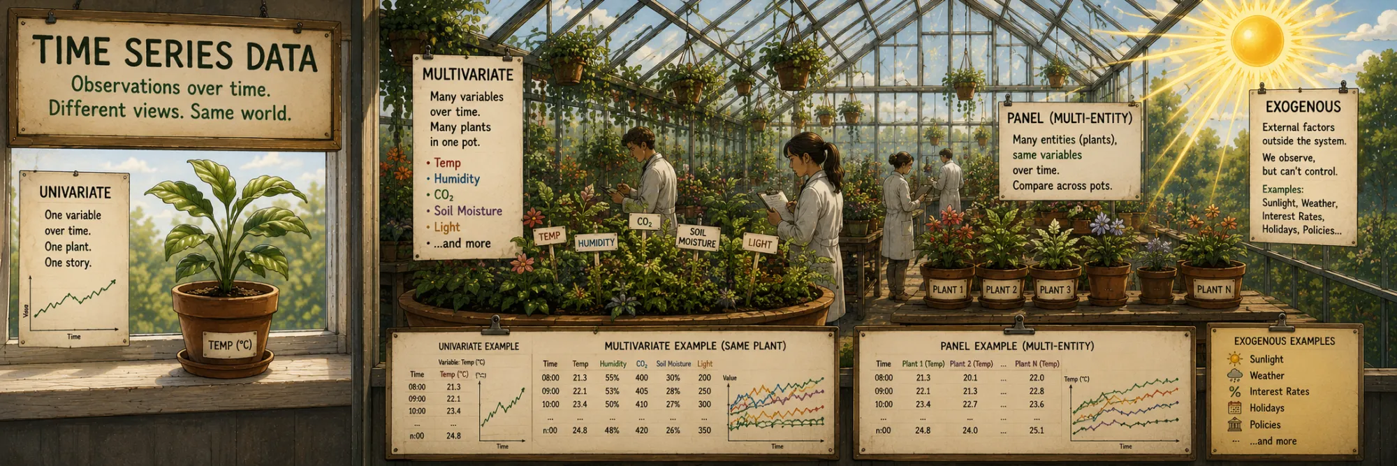
A univariate (one-dimensional) series is a sequence of observations of one variable in time. For each moment in time — one number. The daily closing price of Apple stock, hourly temperature at one point, monthly subscriber count for one product. The structure is (timestamp, value). All classical time series concepts (trend, seasonality, autocorrelation, ARIMA) were originally defined precisely for the univariate case.

A multivariate (many-dimensional, multivariate) series is a sequence of simultaneous observations of several variables in time. For each moment in time — a vector of numbers. Daily closing prices of Apple, Microsoft, and Google simultaneously. Hourly temperature, humidity, and pressure at one point. Monthly revenue, traffic, and conversion rate for one product. The structure is (timestamp, value_1, value_2, ..., value_k).

The key difference is not in the number of columns but in the fact that the variables are potentially related to one another in time. Today's humidity may predict tomorrow's temperature. Apple's and Microsoft's stock prices may co-move, or one may carry predictive information about the other with a lag of hours — without that necessarily implying a direct causal link, since both are also driven by common market factors. These cross-variable dependencies — contemporaneous correlations, lagged effects, and shared latent dynamics — are what true multivariate methods are designed to capture, and what univariate analysis cannot reach by construction.

Three types of "multidimensionality" that get regularly confused

The word "multivariate" in conversations about time series is used for three different situations. This is the central source of confusion — especially when an engineer from an ML team and an engineer from a statistical team discuss the same problem in different words.

Type 1. Univariate with exogenous variables — one target series that we forecast, plus several external predictors (X_1, X_2, ..., X_k) that help make this forecast. Example: we forecast daily sales using product price, weather, and a holiday indicator as external factors. Price, weather, and holiday are exogenous variables — we don't forecast them, we use them. Technically the data has many columns, but this is NOT multivariate in the strict sense — the task has a single target. This is the SARIMAX case. Many practical ML approaches to forecasting end up in the same shape: gradient-boosting on tabular data (LightGBM, XGBoost) builds lag features, rolling statistics, calendar features and known-future covariates, and treats the whole thing as ordinary supervised regression for one target. Neural forecasting models often work with a richer sequence representation rather than collapsing the problem onto a flat feature table — but even then, the conceptual distinction between the target series and the exogenous covariates that help predict it remains exactly the same.

Type 2. Panel (a set of parallel univariate series) — many separate series of identical structure, each with its own target, not necessarily related to each other. Example: daily sales in each of 1000 stores in a chain — these are 1000 parallel univariate series, not a single multivariate series of 1000 variables. A store in Irkutsk and a store in Prague are usually not modeled as variables of one endogenous dynamical system, even though they may well share global drivers such as seasonality, promotions, supply-chain effects or macroeconomic shocks. Those drivers act on every store in roughly the same way; they are not the same kind of mutual feedback that a VAR-style model is built to capture, where today's value of one variable directly feeds into tomorrow's value of another.

Each such series could in principle be forecast with a separate ARIMA, but for thousands of series this is usually inefficient both in compute and in quality — therefore global forecasting models are used (one model trained jointly on all series): DeepAR, TFT, Chronos and other foundation models in general. In ML libraries panel data of this kind is typically represented as a single dataset with item_id and timestamp columns. AutoGluon's TimeSeriesDataFrame, for example, is documented as a collection of univariate time series identified by (item_id, timestamp). Datasets shaped this way are sometimes informally called "multivariate" because they contain many series at once, but conceptually they are still panel (or grouped) time series, not a single endogenous vector that has to be modeled jointly.

Type 3. True multivariate (VAR-style) — several endogenous series forecast jointly, each of which can influence each other. Example: GDP, inflation, unemployment in one country — a macroeconomic system where all three quantities are mutually dependent and move together. We forecast all three simultaneously, modeling their mutual temporal relationships. This is "classical multivariate" from statistics: VAR (Vector Autoregression), VARMA, VECM. There are significantly fewer applications than for the first two types, but in finance, macroeconomics and multi-sensor physical systems this framing is often essential — even when the eventual model is a state-space model, a multivariate neural network or a hierarchical Bayesian system rather than VAR itself, the starting point is the same: a vector of variables that move together over time.

When someone says "I have a multivariate time series" — it's worth immediately clarifying which of the three types is meant. The answer determines which tool to take: SARIMAX and ML for type 1, foundation models or global ML for type 2, VAR/VECM for type 3.

Related terms

A few terms that come up around multivariate time series and that are useful to know right away.

Endogenous vs exogenous variables. Endogenous — variables we forecast (or that the model determines internally). Exogenous — variables we use as known external inputs without forecasting them. In univariate with exogenous — one endogenous variable (y) and many exogenous (X). In the simplest true multivariate case all modeled variables are endogenous, but the boundary is not absolute: practical multivariate systems can also include exogenous covariates, and models such as VARX and VARMAX are exactly the extension of VAR / VARMA in that direction — a vector of jointly modeled endogenous series, with extra known external inputs that influence them but are not themselves predicted.

Cross-sectional vs longitudinal. Cross-sectional data — a snapshot of the state of many units at one moment in time (the salaries of 1000 employees on January 1). Longitudinal (panel) data — the same units at different moments in time (the salaries of 1000 employees by month over 5 years). Time series — a special case of longitudinal data with a focus on a single (or small number of) unit, observed for a long time and frequently.

Lag. A shift in time. If y_{t-1} is the value of the series one step earlier, this is "lag 1". In a multivariate context cross-lag is important: how much series X at moment t-k helps predict series Y at moment t. The analysis of cross-lag (via the cross-correlation function, Granger causality) is the basis of investigating mutual temporal relationships.

Stationarity. A property of a series under which its statistical characteristics (mean, variance, autocorrelation) do not change in time. Most classical methods (ARIMA, VAR) require stationarity or bring the series to it through differencing. Strictly speaking, what these methods require is weak (or covariance) stationarity — a stable mean, variance and autocovariance structure — and not full strict stationarity, which would mean that the entire joint distribution is invariant under shifts in time. In practice, when people discuss ARIMA or VAR, they almost always mean the weak version.