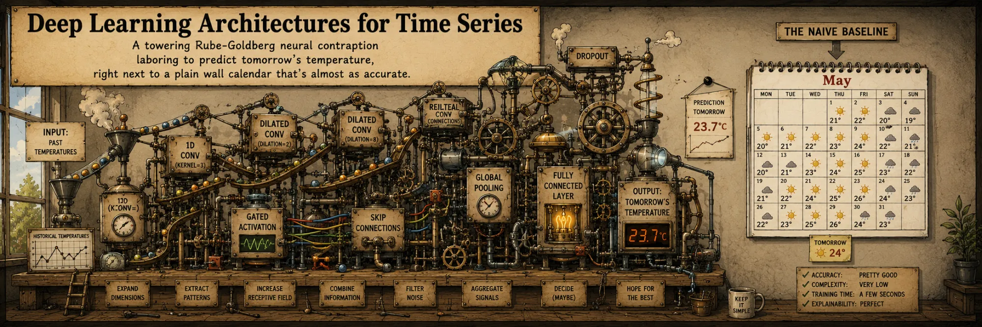
Deep Learning Architectures for Time Series

Between classical statistical models (ARIMA) and modern foundation models (Chronos, TimesFM) lies a layer of deep learning architectures specifically designed for time series: LSTM, TCN, N-BEATS, TFT, DeepAR. Several of them defined the state of practical neural forecasting before the current wave of time-series foundation models, and they gave the impulse for those foundation models in the first place. Even when a new project eventually uses a foundation model — or stays with gradient boosting and statistical baselines, which often remains the right call in business forecasting — understanding these architectures is still useful, because all modern deep learning for sequences stands on their shoulders.

This note is an overview: what each architecture actually is, how its inputs and outputs are shaped, which ones handle multiple input variables, which ones produce probabilistic forecasts (quantiles, intervals, full distributions), and where each tends to fit. The deeper internal mechanics live in their own notes: LSTM and RNN, TCN, one example of a custom hybrid assembly that composes several of these blocks together, and the practical training recipes shared across all of them.

Before going into individual models, it helps to fix the dimensions along which they really differ. Most of the differences boil down to a few practical questions:

• What is the input? A single univariate series, or many parallel series, or a multivariate vector at each time step, or all of the above plus exogenous covariates? A recurring theme in forecasting is honesty about the future: a feature can only be a known-future covariate if it is actually known at prediction time, not just at evaluation time.
• What is the output? A single point forecast for the next step? A full multi-step horizon? A distribution (quantiles, intervals)?
• How much data does it need? Is it designed for one long series, or does it need many related series to learn from?
• What kind of structure is encoded? Pure recurrence, pure convolution, pure attention, decomposition into trend/seasonality, or a hybrid?

The sections below follow roughly the chronological order in which these architectures entered the field — from the founding LSTM through DeepAR and TCN to the forecasting-native N-BEATS and TFT.

A note on local vs global models

One distinction cuts across all of the architectures below and often matters more than the choice of neural block itself. A local model is fitted to one series at a time — one ARIMA per SKU, one LSTM per sensor. A global model is trained jointly on many related series and shares its parameters across all of them. The difference is not architectural — the same LSTM block can be used either way — but it shapes the practical strengths of each model.

A small recurrent network trained globally across thousands of related items can easily beat a sophisticated model trained separately per item, simply because it can share statistical strength across the panel. It is also worth keeping in mind that univariate does not mean single-series: a model can consume one target variable at a time (univariate input window) and still be trained globally across many series. N-BEATS is a typical example on the univariate-window side; DeepAR is a typical example of a global model trained over many related target series. The univariate-vs-multivariate question is about the input sample; the local-vs-global question is about the training set.

A note on multi-step forecasting

Architectures differ not only in what they consume, but also in how they produce a forecast horizon longer than one step. There are three common patterns, and each shows up in the models below.

Recursive (autoregressive) models predict one step, feed that prediction back into the input, and continue stepwise to the end of the horizon. DeepAR is the clearest example: it samples one value, conditions on that sample, and rolls forward. Recursive forecasting is conceptually clean and naturally extends to arbitrary horizons, but errors accumulate — a small mistake at step 1 distorts the input for step 2, and the bias compounds.

Direct (multi-horizon) models output the entire forecast vector in a single forward pass from the input window. Vanilla N-BEATS works this way: a fixed lookback in, a fixed horizon out, with no feedback loop. Direct forecasting avoids feedback drift and tends to produce smoother long-horizon outputs, but the model has to learn the whole horizon shape in one shot, and adding even one extra horizon step usually means re-training.

Encoder-decoder models sit in between: an encoder summarizes the past, a decoder emits future steps sequentially while consuming any known-future covariates as it goes. TFT and seq2seq LSTM forecasters use this pattern. It keeps the flexibility of stepwise output (for using future-known features at each future step) while avoiding the strict closed-loop autoregression that compounds error from the model's own predictions.

This distinction matters because two architectures with very similar building blocks can produce very different multi-horizon behavior depending on which of these three patterns they use.

---

LSTM (Hochreiter & Schmidhuber, 1997)

LSTM is a classical recurrent neural network, invented by Hochreiter and Schmidhuber in 1997. For many years it was one of the default neural choices for sequence modeling, including time series. LSTM processes a sequence element by element, maintaining internal state (hidden state and cell state), which allows it to remember long-range dependencies. The deep dive into the cell, the gates, and the cell state lives in its own note; here we look at LSTM as a forecasting architecture rather than as a layer.

Architecture

In its most common forecasting form, LSTM is wrapped in an encoder-decoder seq2seq pattern: the encoder consumes a fixed lookback window of the past and compresses it into a hidden state, the decoder emits the forecast horizon step by step. For short horizons, a simpler "many-to-one" form (LSTM reads the past, a final dense layer outputs the next H values jointly) is often used and is faster to train.

LSTM has a theoretically unbounded receptive field, but in practice very long-range dependencies are hard to learn reliably — gradients and useful signal still dilute over long sequences even with the gating mechanism. For longer-range dependencies LSTM is typically combined with attention (see hybrid composition below), or replaced outright with attention-based models.

Inputs and outputs

LSTM happily consumes multivariate inputs at each time step: instead of a scalar x_t, you feed a vector. That is the standard way to add exogenous covariates — just stack them as additional input channels alongside the target. Static covariates (country, product type) are usually broadcast across time or fed through a separate embedding.

Vanilla LSTM produces point forecasts. Probabilistic outputs are added by changing the head: an output layer that produces parameters of a distribution (mean and variance for Gaussian, μ and σ for log-normal), or several quantile outputs trained with quantile loss. None of this is built in — it is a deliberate architecture choice on top.

When it tends to win

LSTM is rarely the strongest model on any single benchmark today, but it is still a reasonable starting point when you need a flexible neural baseline that handles multivariate inputs naturally, or when the deployment target has tight memory/latency constraints (LSTM has a small footprint compared to attention-based models). In modern production it is more often used as a component inside larger architectures (see DeepAR below, and the bespoke hybrid assembly walked through separately as one example) than as a standalone model.

---

DeepAR (Amazon, 2017)

DeepAR is an influential global LSTM-based forecasting model from Amazon, released in 2017. It became one of the most influential industrial baselines for probabilistic forecasting of many related series, and it pioneered many of the ideas that foundation models later generalized. It is not itself a foundation model — it is trained on your forecasting panel, not pre-trained once on a large external collection of time series.

What it is

The main difference between DeepAR and classical approaches is that it trains on a set of similar series simultaneously, rather than on each series separately. If you have 1000 product SKUs and each has its own time series of sales, classical ARIMA fits 1000 separate models. DeepAR fits one large RNN model on all of them at once. This gives the model the ability to transfer knowledge between series — if one product has a similar seasonality to another, the model notices and uses it. The same logic as foundation models, but on a smaller scale: DeepAR learns from your panel of related series.

Architecture

Technically, DeepAR is an autoregressive RNN:

• An LSTM or GRU processes the sequence of past values (plus optional covariates).
• A likelihood layer (Gaussian for continuous data, Negative Binomial for counts) outputs the parameters of the distribution for the next step, rather than a point estimate.
• Training is by maximum likelihood: the model tries to assign high probability to the actual observed values.

For forecasting at inference, the model samples from the predicted distribution, continues autoregressively for the full horizon, and collects multiple sample paths. Quantiles and prediction intervals are obtained from those sample paths — DeepAR is a fully probabilistic model by design, not as an afterthought.

Inputs and outputs

DeepAR consumes a panel of related series (the practical lower bound is usually a few dozen series of sufficient length), with an item_id per series so the model knows which examples belong together. Each series can have its own exogenous covariates (past observed and known future), and static covariates per item are passed through embeddings. Outputs are probabilistic at every horizon step, with whatever quantiles you need read off the sample paths.

When it tends to win

DeepAR is a good choice when you have many related series with enough history each, and you care about probabilistic forecasts — for example, demand forecasting across thousands of SKUs, traffic forecasting across many endpoints, energy load forecasting across substations. It can be weaker than foundation models in cold-start settings — a brand-new or very short series — especially when the item-level history is too short for the model to infer its own pattern; a pre-trained foundation model may already contain useful generic forecasting priors and need less per-item history. Static covariates and category embeddings can soften the cold-start problem somewhat, but a genuinely new item is still harder for DeepAR than for a zero-shot foundation model. Conversely, DeepAR usually fares well when there is plenty of historical data and the team prefers a more controlled, less black-box solution than a foundation model.

---

TCN — Temporal Convolutional Network (Bai, Kolter, Koltun, 2018)

TCN is the convolutional alternative to recurrent networks for sequence modeling. It showed that for a wide range of sequence tasks, properly designed 1D convolutions can match or beat LSTMs, while training in parallel and avoiding many of the gradient issues that recurrence suffers from. The detailed mechanics of causal convolution, dilations and residual connections live in the TCN note; here we look at it as a forecasting architecture.

Architecture

A TCN forecasting model is a stack of causal dilated 1D convolutions: each layer uses a kernel that only looks at the past (causal padding), and dilations grow exponentially with depth so that a few layers cover hundreds of past time steps. Add residual connections, normalization or dropout, and sometimes gated activations such as GLU between blocks, and you have a strong sequence model. (The original TCN of Bai et al. uses ReLU; gating is a common hybrid extension rather than a canonical part of the architecture.)

Inputs and outputs

Like LSTM, TCN takes a sequence of vectors per time step, so multivariate inputs are supported naturally — every input channel becomes an extra input dimension to the convolution. Static covariates can be broadcast across the time axis or handled by a separate dense pathway.

Vanilla TCN produces point forecasts for the chosen horizon. Probabilistic versions follow the same pattern as LSTM: replace the output head with one that emits distribution parameters or multiple quantiles.

When it tends to win

TCN is the natural choice when you want fast parallel training on long sequences — it is often easier to train efficiently than LSTM on long context windows because there is no inherent sequential dependency through the layer. It also tends to be more stable to train, since vanishing gradients are less of an issue with residual conv stacks than with recurrence. Practical forecasting systems often use TCN as a feature extractor in front of an LSTM or attention block (the hybrid pattern), getting fast initial extraction plus the temporal sharpness of recurrence on top.

---

N-BEATS (Element AI, 2020)

N-BEATS (Neural Basis Expansion Analysis for Time Series) is a model from Element AI that achieved state-of-the-art results on the M4 forecasting benchmark, showing that a pure neural architecture could compete with strong statistical and hybrid methods. What's unusual about N-BEATS is that it's a pure fully-connected network — no recurrent or convolutional elements at all.

Architecture

The architecture is a stack of blocks, where each block predicts a part of the input (the backcast) and a part of the output (the forecast). The backcast prediction is then subtracted from the input before passing it to the next block, so each subsequent block models only the residual that the previous blocks could not explain. This is iterative residual learning of the time series itself, not of the loss surface — closer in spirit to gradient boosting than to ordinary deep learning.

In the interpretable variant, blocks are constrained to use specific basis functions: polynomials for trend blocks, Fourier series for seasonality blocks. The output then naturally decomposes into trend + seasonality + residual components, which is human-readable. In the generic variant the basis is unconstrained, the network learns it from data, and accuracy is usually somewhat higher at the cost of interpretability.

Inputs and outputs

N-BEATS expects a fixed-length univariate input window (the lookback window) and produces a fixed-length forecast horizon. The lookback is typically several times the horizon (a common starting point is 3–7× the horizon length).

The vanilla N-BEATS does not support multivariate inputs or exogenous covariates: each input sample is a single series of values. There is a follow-up called N-BEATSx (Olivares et al., 2022) that adds support for known-future and historical covariates; it is a direct extension and is what you reach for if you need exogenous variables in the same architecture.

The vanilla model produces point forecasts. Probabilistic versions exist via training with quantile losses or by ensembling many runs, but they are not part of the original formulation.

When it tends to win

N-BEATS is unusually strong as a univariate neural baseline: each training example is a single target window, without explicit multivariate covariates. It can be trained on one long series or globally across many related univariate series, but vanilla N-BEATS does not consume a multivariate feature vector at each time step. It tends to perform well on M4-style benchmarks and on demand-forecasting series with strong seasonal patterns, while staying conceptually simpler than recurrent or transformer architectures. When the data has rich heterogeneous covariates and you need them inside the model (rather than as a preprocessing step), TFT or one of the global models above is usually a better fit.

N-BEATS demonstrated an important thing: for time series, it is not necessary to use RNNs — deep fully-connected networks are enough if structured correctly. This helped make the field more comfortable with architectures that are not recurrent by default.

---

TFT — Temporal Fusion Transformer (Google, 2020)

TFT from Google Research is an attention-based architecture specifically designed for forecasting with a rich set of inputs. Where N-BEATS deliberately strips the inputs down to a single series, TFT goes the other way — it is built to digest as many heterogeneous inputs as you can give it, and to do so transparently.

Architecture

TFT explicitly separates inputs into several categories and processes each through its own pathway:

• Static covariates — features that do not change over time (product category, region, sensor type).
• Known future inputs — values known in advance for the forecast horizon (planned promotions, scheduled holidays, calendar variables).
• Observed past inputs — historical values of the target and any past-only covariates (past weather, past sales).

Each input passes through a Variable Selection Network (VSN), which learns per-step importance weights so that irrelevant features are softly suppressed. The selected features go through a sequence-to-sequence LSTM encoder (for past) and decoder (for future), and then through a multi-head temporal attention layer that lets the model attend across the whole context. Quantile forecasts come out of the final dense head.

A defining feature of TFT is interpretability: the attention weights and the variable-selection weights are both directly inspectable. You can read off which past time steps the model attended to for a given prediction, and which features the variable-selection network considered important when. These weights are useful diagnostic signals, but they should not be treated as perfect causal explanations — they describe how the model routed information internally, not necessarily which variables truly caused the forecast. With that caveat, TFT is still much more transparent than most neural forecasters, which is often the deciding factor for regulated industries (healthcare, finance).

Inputs and outputs

Inputs are explicitly multivariate: TFT was designed from the start to handle a heterogeneous mix of static, past-only, and future-known features simultaneously, with each category routed through its own pathway rather than concatenated blindly.

Outputs are probabilistic out of the box: the standard formulation produces multi-quantile forecasts (e.g. p10/p50/p90), via a quantile loss. This makes uncertainty estimation a first-class feature, not something bolted on.

Data preparation involves splitting the input columns into the three categories (static / past / known-future) and feeding them to TFT as separate tensors — a step that requires being honest about what is actually known at prediction time.

When it tends to win

TFT shines on forecasting with many heterogeneous inputs: retail demand with calendar, weather, promotions; energy with weather forecasts and tariffs; healthcare with patient covariates. It also shines whenever quantile forecasts and interpretability are both required. It is heavier than N-BEATS or pure LSTM and rarely the right choice for a quick single-series baseline.

---

Building hybrid architectures

In practice, a single architecture from the list above is often not the final form of the production model. Each of these blocks — LSTM, TCN, attention, decomposition heads, embeddings — has its own strengths, and they compose well. A typical hybrid for tabular-style forecasting might run a TCN over the input window for fast feature extraction, pass the result through an LSTM for sharper local recurrence, add a multi-head attention layer on top for long-range dependencies, and finally split the output into separate trend / seasonality / residual heads in the N-BEATS spirit. Calendar features go through embeddings, exogenous variables go through their own pathways, known-future covariates are fed only to the decoder.

There is no single "correct" hybrid; it is a design space rather than an architecture, and most production systems end up with some combination tuned to their data. The point of knowing all the building blocks individually is exactly that — to be able to reach for the right one when designing or debugging the network. The same ideas underpin TFT, DeepAR, and the foundation models that came later; they are just frozen at different points in the design space.

---

Comparison

A compact summary of the architectures in this note along the dimensions that matter most when picking one:

Model	Backbone	Multivariate inputs	Probabilistic output	Designed for	Practical strength
LSTM	Recurrent (gated)	Yes (vector per step)	No by default; add a distribution head	General sequence modeling	Flexible component, small footprint
DeepAR	Autoregressive LSTM/GRU + likelihood head	Yes (per-item covariates + static embeddings)	Yes (samples from learned distribution)	Many related series, panel data	Probabilistic by design; transfers across related series
TCN	Causal dilated 1D convolution	Yes (channels per step)	No by default; add a distribution head	Long-context sequence modeling	Parallel training; stable on long contexts
N-BEATS	Stacked MLP with backcast/forecast residuals	No (univariate input sample; use N-BEATSx for covariates)	No (point forecast); quantile via training loss	Univariate target window; can train local or global	Strong univariate baseline; interpretable trend / seasonality decomposition
TFT	LSTM encoder-decoder + attention + VSN	Yes (static, past, future-known explicitly separated)	Yes (multi-quantile by default)	Forecasting with rich heterogeneous inputs	Interpretable; quantiles built in

---

When each tends to win

The choice between these architectures is rarely about one being "better" in the abstract — it is about whether the shape of the data and the requirements of the forecast match what each model was designed for.

• One long, well-behaved univariate series: N-BEATS is usually the strongest neural baseline. ARIMA/SARIMA is a simpler alternative worth running first.
• One series with rich heterogeneous covariates and a need for quantile forecasts and interpretability: TFT is the natural fit.
• Many related series with enough history each, probabilistic forecasts wanted: DeepAR.
• Many related series, very short history per series, no time to retrain regularly: foundation models (Chronos, TimesFM) — their pre-training often gives them an edge on cold start that DeepAR cannot match without your own panel.
• Long input contexts where training time matters and the architecture should parallelize well: TCN, possibly as a feature extractor in front of an LSTM or attention layer.
• A general-purpose flexible neural baseline you intend to combine with other blocks: LSTM remains useful, even though as a standalone model it has been overtaken by all of the above on most benchmarks.

For most teams the reasonable working order in tabular business forecasting is: start with a classical statistical baseline, then a global gradient-boosted baseline (LightGBM, XGBoost or CatBoost with lag, rolling, calendar and known-future features) — this is often the strongest non-neural baseline and frequently competitive with anything heavier — then a foundation model zero-shot, then — if the data really warrants it — train DeepAR, TFT or N-BEATS on the panel. A bespoke custom hybrid built out of these blocks (one such assembly is walked through separately) is a fully reasonable destination, but it is rarely the right first destination.

This order is not a law; it is a pragmatic exploration order when you want quick baselines before committing to a heavier training pipeline. For teams with mature panel data, established training infrastructure, and tight latency or compliance requirements, training a global DeepAR/TFT first — or sticking with a well-tuned gradient-boosted model — may be the right move, and a foundation model is the experiment rather than the default. The point of the workflow is to anchor expectations cheaply, not to prescribe a fixed sequence.