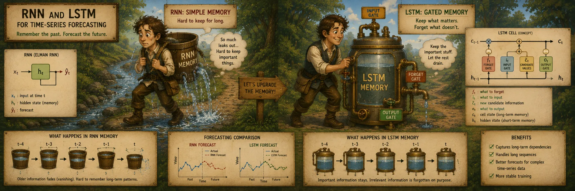
RNN and LSTM for Time-Series Forecasting

This note walks through the recurrent backbone behind most pre-foundation-model time-series deep learning: vanilla RNN, the vanishing-gradient problem that makes long-range dependencies hard to learn in practice, and LSTM as the gated response to that problem. It is a companion to the architectures overview — that one places LSTM next to TFT and N-BEATS at a high level; here we go inside the LSTM cell itself. The components introduced here are the foundation for many bespoke hybrid forecasting assemblies people put together (one such assembly is walked through separately) and reuse the training recipes (initialization, dropout, etc.) discussed in their own note.

---

RNN — the foundation upon which LSTM is built

Before discussing LSTM, it's worth understanding the vanilla RNN — the architecture from which LSTM grew as a solution to its problems. RNN is a classic that appeared in the 1980s, but it's still conceptually important for understanding all subsequent evolutions of recurrent neural networks.

A Recurrent Neural Network is a neural network for sequential data. It processes a sequence x_1, x_2, ..., x_T one element at a time, maintaining a hidden state h_t that accumulates information about the past.

The fundamental idea of an RNN is recurrence. A classic feedforward network takes a fixed-size input and produces a fixed-size output, with no memory between calls. An RNN, on the other hand, processes a sequence step by step, maintaining an internal state (hidden state) that changes after each step. At each step, the network sees the current input plus the previous hidden state, and uses both to update the hidden state and form the output.

Thanks to this, an RNN can process sequences of any length and maintain context between steps.

Vanilla RNN formula

h_t = tanh(W_h × h_{t-1} + W_x × x_t + b)
y_t = W_y × h_t

Mathematically, a vanilla RNN is structured very simply. The hidden state h_t at step t is computed as a nonlinear function (usually tanh) of the combination of the previous hidden state h_{t-1} and the current input x_t, multiplied by learned weight matrices W_h and W_x. The output y_t is a linear function of the hidden state.

All matrices are shared between steps — this is parameter sharing, which gives the RNN the ability to generalize to sequences of any length. Despite the simplicity of the recurrence, RNNs are theoretically very expressive; the practical difficulty is not expressiveness, but training them reliably over long sequences.

The vanishing / exploding gradient problem

The main practical problem of vanilla RNN is vanishing/exploding gradients during training.

Training happens via backpropagation through time (BPTT) — an extension of ordinary backprop to recurrent connections. To compute the gradient with respect to h_0 (the hidden state at the start of the sequence), you need to "unroll" the RNN over its entire length and run backprop through every step. In doing so, the gradient is multiplied by W_h at each step backward.

More precisely, the gradient depends on a long product of Jacobians at each unrolled step (containing W_h, the derivative of tanh, and the activations themselves), and the behavior of that product is what matters. The consequences:

• If the repeated Jacobian products have effective scale below 1, the gradient decays exponentially — the model cannot learn dependencies longer than a few steps.
• If their effective scale is above 1, the gradient grows exponentially and explodes — NaN in the weights, training blows up.

A useful simplified intuition is to think of repeatedly multiplying by the recurrent matrix W_h: if its eigenvalues are below 1 in magnitude, gradients shrink; if above 1, they blow up. Keeping this effective scale stable across many unrolled steps is difficult. For short, simple sequences vanilla RNNs can still work — the architecture is not mathematically useless. The problem is that real forecasting often requires learning dependencies across many time steps, and vanilla RNNs make those dependencies hard to train reliably. That difficulty is what motivated the development of LSTM.

The solution — gating mechanism

The standard response to the vanishing-gradient problem in recurrent networks is a gating mechanism: gates that explicitly control the flow of information (and the gradient) through time steps. Two architectures dominate the family:

• LSTM (Long Short-Term Memory), Hochreiter & Schmidhuber, 1997 — the first successful architecture with gating. Maintains a separate cell state C_t in addition to the hidden state h_t, and uses three gates (forget, input, output) to control what flows in and out of it.
• GRU (Gated Recurrent Unit), Cho et al., 2014 — a simpler gated recurrent architecture. It has gates (update and reset) as well, but it does not maintain a separate cell state. Instead it updates the hidden state h_t directly through those gates, which makes it lighter than LSTM and often comparable in practical performance.

Either way, sigmoid-activated gates (vectors between 0 and 1) multiplicatively decide what information passes through. This does not magically remove the difficulty of learning long-range dependencies, but it gives the model a much more stable gradient path through time: when the relevant gate stays close to 1, information and gradients can pass across many steps with much less decay than in a vanilla RNN.

---

LSTM — Long Short-Term Memory

The cell state idea

The central idea of LSTM is to split "memory" into two components:

• h_t (hidden state) — for short-term computations, visible to the outside.
• C_t (cell state) — for long-term memory, hidden.

C_t passes through time steps with minimal modification — not through a nonlinearity at every step, like in vanilla RNN, but through additive updates. This makes LSTM a "superhighway" for information when it needs to be preserved for a long time.

Control over what and how C_t is modified is exercised through gates — vectors from [0, 1], obtained via sigmoid, which multiplicatively manage the flow of information. There are three gates total: forget, input, and output.

Forget gate — what to throw out of memory

f_t = σ(W_f × [h_{t-1}, x_t] + b_f)

The forget gate decides what part of the previous cell state to keep, and what to forget. The sigmoid produces a vector of the same size as C_t, with values between 0 (completely forget) and 1 (completely keep).

Based on the current input x_t and the previous hidden state h_{t-1}, the model learns: "seeing this combination, I should forget feature 5, keep feature 7, partially keep feature 2". This is a key mechanism: vanilla RNN cannot selectively forget, but LSTM can.

Input gate — what to write into memory

i_t = σ(W_i × [h_{t-1}, x_t] + b_i)
C̃_t = tanh(W_C × [h_{t-1}, x_t] + b_C)   # candidate values

The input gate, in parallel, decides what new information to write into the cell state. The process consists of two parts:

• i_t — the gate itself, a sigmoid vector that determines "how important it is to record each of the candidates".
• C̃_t — candidate values, passed through tanh (values in the range [-1, 1]) — possible additions to the cell state based on the current input.

Their elementwise multiplication gives gated values that will be added to C_t.

Cell state update

C_t = f_t * C_{t-1} + i_t * C̃_t
     \____forget___/   \___add new___/

The cell state update formula is the heart of LSTM. The first part — f_t * C_{t-1} — is the old cell state passed through the forget gate (elementwise multiplication). The second part — i_t * C̃_t — is new information passed through the input gate. The sum of these two is the new cell state.

It's important that this is an additive update, not a fully multiplicative pass through a weight matrix as in vanilla RNN — that is what gives LSTM a much safer gradient path through time.

Output gate — what to give to the outside

o_t = σ(W_o × [h_{t-1}, x_t] + b_o)
h_t = o_t * tanh(C_t)

The output gate controls which part of the cell state is used to form the hidden state (which is what's given to the outside as the output of this step).

The sigmoid o_t determines which features of C_t to "open" for output. The new h_t is C_t passed through tanh (in [-1, 1]) and multiplied by the output gate.

The separation of cell state and hidden state is important: the cell state can hold complex information, but the output is only a relevant subset for the current moment.

Why LSTM mitigates vanishing gradient

The key property of LSTM that addresses vanishing gradient: the cell state C_t receives a direct additive gradient path from C_{t-1} to C_t.

During BPTT, the gradient from C_{t+1} to C_t is simply multiplied by f_t (a vector in [0, 1]), not by a whole weight matrix with exponential risks. If the model learns f_t = 1 (keep), the gradient passes through almost unchanged. This is called the constant error carousel — the gradient can "ride" through many time steps with much less decay or explosion than in a vanilla RNN. When the forget gate stays well below 1 the gradient still attenuates, so this is mitigation rather than a magical fix; but it is enough to make a fundamental difference in what the network can learn.

This is why LSTM can learn substantially longer dependencies than a vanilla RNN in practice. The exact range is data- and architecture-dependent, and very long contexts are still difficult without attention, convolutional shortcuts, or other architectural help.

LSTM in Keras

x = layers.LSTM(
    lstm_units,                  # hidden state size
    return_sequences=True,       # return h_t for all steps
    dropout=dropout_rate,
    kernel_initializer=GlorotUniform(seed=42),      # W_x init
    recurrent_initializer=Orthogonal(seed=42),      # W_h init
)(sequence_input)                # input tensor (batch, window_size, n_features)

lstm_units — the dimensionality of the hidden state and cell state (typically 64–256). return_sequences=True — return hidden states for all time steps, not just the last one (needed for attention or another recurrent layer on top). dropout — dropout applied to the input transformation at each time step, used as regularization. Keras also exposes recurrent_dropout for the recurrent state-to-state connection, which is theoretically more correct but in practice often slows training because it disables some optimized cuDNN kernels — see the training recipes note for the full discussion. The initialization is also worth noting: kernel_initializer=GlorotUniform for input weights (W_x), recurrent_initializer=Orthogonal for recurrent weights (W_h) — the why of those choices is in the same note.

---

Shapes for time-series forecasting

For forecasting, the input to an LSTM usually has the shape:

(batch_size, window_size, n_features)

where window_size is the lookback length and n_features includes the target value and any optional covariates at each time step. The output shape depends on return_sequences:

return_sequences=False  →  (batch_size, lstm_units)
return_sequences=True   →  (batch_size, window_size, lstm_units)

The first form gives you a single summary vector after the whole sequence has been read; the second gives you a hidden state per time step. Which one to use depends on what comes next.

return_sequences=True — why and when

The return_sequences parameter is an important practical detail of working with LSTM in Keras that often confuses beginners. By default, Keras LSTM returns only the last hidden state h_T after processing the entire sequence — useful for classification tasks (read sequence → classify) or for any setup where one summary vector is all you need.

For multi-step forecasting with horizon > 1, returning only the last hidden state can still work perfectly fine: a Dense head on top of h_T can output the entire horizon vector in one shot (Dense(horizon)(h_T)). This is the direct multi-output pattern, and it does not require return_sequences=True.

What return_sequences=True is really for is the case where the next layer needs access to the whole encoded sequence rather than to a single summary vector — for example:

• another stacked LSTM layer that will run over the same sequence again;
• a multi-head attention layer that has to attend over past steps;
• a TimeDistributed head that emits one output per past step;
• a sequence-to-sequence decoder that attends over the encoder states.

In all of those cases the full per-step tensor (batch, window_size, lstm_units) is needed and return_sequences=True is the way to get it. Outside those cases the default (just h_T) is usually enough.

---

LSTM forecasting patterns

In forecasting, LSTM almost always appears in one of three patterns. They map directly onto the multi-step categories from the architectures overview (recursive vs direct vs encoder-decoder), and choosing the right one usually matters more than tuning the hidden-state size:

1. Many-to-one. Read a window of the past, predict a single value (the next step, or some scalar summary of the horizon). The encoder uses return_sequences=False, the head is a small Dense(1). The simplest pattern, useful when the natural problem is "predict the next value" or when a separate downstream model handles the horizon.
2. Many-to-many direct. Read a window of the past and output the full horizon vector in one shot. Same encoder as above (return_sequences=False), but the head is Dense(horizon). This is the direct multi-output pattern from the overview — no autoregressive feedback loop, no error accumulation across the horizon.
3. Encoder-decoder (seq2seq). An encoder LSTM consumes the past and summarizes it; a decoder LSTM emits future steps sequentially, optionally conditioning each step on known-future covariates and on its own previous output. In a simple seq2seq setup without attention, the encoder may pass only its final state to the decoder (return_state=True). If the decoder or an attention layer needs access to all encoded time steps, the encoder uses return_sequences=True instead. This is the natural pattern for long horizons with rich covariates and attention-based recurrent forecasters, and it is close to the recurrent backbone used in TFT-style architectures. DeepAR uses a related pattern, but it is more strictly autoregressive and produces sample-based probabilistic forecasts via a likelihood head rather than emitting a horizon vector directly.

Most practical LSTM forecasters live in pattern 2 or 3. Pattern 1 is more common in monitoring-style "predict the next value" use cases and in research code; for end-to-end horizon forecasting, direct multi-output or encoder-decoder is usually the better default.

A practical note on LSTM for forecasting

LSTM is flexible, but it is not automatically a better forecasting model than ARIMA, gradient boosting, TCN, TFT, or foundation models — and on its own it is rarely the strongest option on modern benchmarks.

Its main practical value today is as a compact recurrent building block: useful for capturing local temporal dynamics, easy to combine with covariates by stacking them as extra input channels, small in memory footprint, and still common as a component inside all kinds of custom hybrid forecasting assemblies and inside DeepAR-style global probabilistic models. Treat it as a known-quantity recurrent module that you reach for when something specific in your pipeline benefits from it, not as the default forecasting model on its own.