Chapter 2 of 5

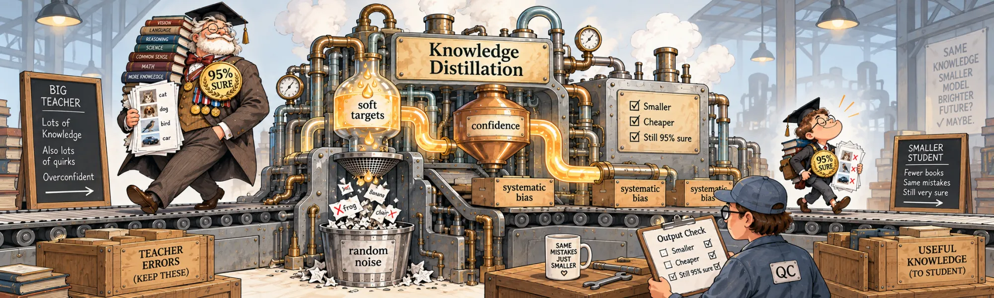
Knowledge Distillation: What a Teacher Actually Teaches

Created Apr 28, 2026 Updated Sep 18, 2026

See the lab — real experiments from this note

Show a well-trained classifier a photo of a cat and it answers cat, which is usually the only part of the answer anyone looks at. What the network actually produced is ten numbers, one for every class it knows: something like 80% cat, 12% dog, 5% deer, a sliver for bird and almost nothing for truck. The label in the training set said only cat. The network's answer says more — that this particular cat looks a bit like a dog, not at all like a truck, and that the network is not completely sure about it.

Now train a second, much smaller network on those ten numbers instead of on the label, and that is knowledge distillation. The big network is the teacher, the small one is the student, and the student learns to answer the way the teacher answers. DistilBERT was made from BERT this way, and the small Gemma 2 and Llama 3.2 models learned from their bigger siblings the same way. Long before any of them, whole ensembles of models were being squeezed into a single one with the same trick.

At first sight it is not clear why this should help. The labels are the right answers, while the teacher is a model that makes its own mistakes — the one in this note gets about one test photo in sixteen wrong. Swapping the right answers for a fallible model's opinions sounds like a downgrade. And yet a network with 24 thousand parameters gets 77.7% of the test photos right when it learns from the labels, and 79.9% when the same network learns from the teacher's answers.

So the teacher passes on something the labels do not have, and it is not obvious what that is. It could be nothing more than softness: a target of 80% is gentler than a target of 100%, gentler targets are known to help, and then any softened label should work as well as the teacher. It could be the teacher's sense of which classes are alike, that cats sit nearer to dogs than to trucks, and then keeping the softness but scrambling which classes get it should throw the gain away. And if it really is knowledge, a whole chain of consequences follows. A bigger teacher should teach more, copying its insides should teach even more, the student should never beat its teacher, and whatever the teacher got wrong should come along with the rest.

All of these guesses can be checked on real networks. Some of them hold up, and a few fall apart in ways that say more about distillation than the ones that hold.

The note goes in four steps. First, what a teacher's answer contains and which part of it actually helps — including when the labels it learned from were wrong. Then what can be varied around it: the teacher, what is copied from it, how long the student trains, and above all which questions the teacher is asked. Then what travels badly: the difference between copying a teacher and being right, and the mistakes and overconfidence that come along with the knowledge. Finally, language models, and whether any of this pays for its compute.

What a teacher's answer contains

A classifier's last layer produces one number per class, a logit $z_k$ . The softmax turns logits into probabilities:

p_k = \frac{e^{z_k / T}}{\sum_j e^{z_j / T}}.

Normally $T = 1$ . A well-trained network then puts almost all of its probability on one class, and the rest is spread over numbers so small they look like rounding. They are not rounding. The logits behind them are perfectly ordinary numbers, and their order says which wrong answers the network considers nearly right. Dividing by a temperature $T > 1$ shrinks the differences between logits and makes that order visible.

The teacher in the widget below, and in most of this note, is a convolutional network of the ResNet family with 4.3 million parameters. It was trained from scratch on CIFAR-10 — small colour photos, 32×32 pixels, of ten classes: airplane, automobile, bird, cat, deer, dog, frog, horse, ship, truck. It learned from the 50,000 labelled training photos, for 30 passes over them, each time shown with random crops and mirror images, and it gets 93.7% of the 10,000 test photos right. Those test photos are never used for training by any model in this note, and every accuracy quoted is measured on them.

Pick almost any image and the pattern is the same. At $T = 1$ the teacher is close to certain. At $T = 4$ the other classes appear, and they are not random. Averaged over the whole test set, the classes the teacher considers closest to automobile are truck and ship; to cat, dog and bird; to horse, dog and deer; to airplane, bird and ship. Nobody told it that. It learned the resemblance from pixels, and it will tell a student.

This information is often called dark knowledge: it is in the model, it is used by the model, and it never appears in the model's top-1 answer. A training label cannot carry it, because a label has nowhere to put it. A teacher's full distribution can.

How a student learns from a teacher

The student in most of this note is a plain three-layer convolutional network with 24 thousand parameters, nearly two hundred times smaller than the teacher, and trained on the labels alone it gets 77.7% of the test photos right. Distilling it takes two stages. First the teacher looks once at every training photo and at its mirror image, and its ten logits for each of them are written down; after that the teacher is not needed any more. Then the student trains in the ordinary way — 6,000 steps, about 30 passes over the data, 256 photos at a time — except that for each photo, instead of the label, it is given the teacher's ten numbers for that photo. Both the student's numbers and the teacher's are softened with the same temperature, the loss measures how far apart the two distributions are, and each step nudges the student's weights so that its answer about that photo moves toward the teacher's. At no point does the student see how the teacher works inside, only what it answered.

Written as a formula, the loss most implementations use mixes the label and the teacher:

\mathcal{L} = \alpha \, \mathrm{CE}\big(y,\; q\big) \;+\; (1 - \alpha)\, T^2\, \mathrm{KL}\big(p_T \,\|\, q_T\big),

where $q$ is the student's distribution, $p_T$ and $q_T$ are teacher and student softened at the same temperature, and $\alpha$ weighs the label against the teacher. The $T^2$ is bookkeeping: softening both distributions by $T$ shrinks the gradient of the KL term by about $T^2$ , and multiplying it back keeps the two terms comparable as the temperature changes. In the limit of a very high temperature the KL term turns into something plainer still — matching the student's logits to the teacher's with a squared error, once both are centered, each shifted so that its ten logits average to zero.

Cross-entropy and KL are the same objective here. The KL divergence splits into two pieces:

\mathrm{KL}(p \,\|\, q) = \underbrace{\sum_k p_k \log p_k}_{-H(p)} \;-\; \sum_k p_k \log q_k = \mathrm{CE}(p, q) - H(p).

The teacher's entropy $H(p)$ does not depend on the student at all. So training a student with the KL divergence and training it with cross-entropy against the teacher's probabilities is the same optimization: identical gradients, losses that differ by a constant. Computed on random logits, the two gradients differ by $2 \times 10^{-9}$ — float rounding — and the two losses differ by exactly $T^2 H(p)$ , to six decimal places. Nothing about the loss is specific to distillation. It is ordinary cross-entropy, pointed at a soft target instead of a one-hot one — the same cross-entropy the training note derives from maximum likelihood.

How the numbers were measured. Every experiment in this note runs in one notebook, the lab linked with it, on the GPU of an Apple M3 Max; the whole lab takes about five hours.

Training. Every image model trains with SGD (Nesterov momentum 0.9, weight decay $5 \times 10^{-4}$ , batch 256) under a one-cycle learning-rate schedule peaking at 0.1. Teachers train for 30 passes with random crops and mirror images; students for 6,000 steps, about 30 passes, with mirror images only unless a section says otherwise, and a label-trained student always gets exactly the same budget as the distilled one it is compared with.
Runs. Every configuration is trained three times from different seeds — twice for the longest runs: the training budgets, the warm start, the transfer-set fractions, the larger student on noisy labels and the language models. A seed fixes the initial weights, the order of the data and the augmentation, so the same configuration run twice gives the same numbers up to the GPU's own nondeterminism. The text quotes means; the widgets show the spread.
Resolution. Identical configurations repeated in different experiments land within about 0.3 of a point of each other, and differences smaller than that are treated as no difference.
Evaluation and tuning. Every accuracy is on the 10,000 test photos, which no model ever trains on. There is no separate validation set, and the temperature and label weight used throughout were chosen by looking at test accuracy; the choice matters modestly (temperature 4 beats 8 by 0.6 of a point and 2 by 1.3), but it was made on the test set.
What was planned. The ladder, the teachers, features, the direction of the KL divergence, the transfer data, born-again networks, inherited flaws, fidelity, language models and the cost were planned together. Noisy labels, the training budget, the view the teacher is asked about, the choice of transfer images and the student's size were added in a second round, after the first results were in.
The running example. The twelve photos that recur through the note come from separate training runs of the same setup, so the accuracies in those widgets can differ from the text by up to the resolution above.

Why a teacher can teach better than the labels

There are at least three different explanations of why soft targets help, and they are usually run together.

More information per example. A label is one class. A distribution is ten numbers: how sure the teacher is about this image, and which wrong classes are close.
Regularization. Any soft target asks the student for less than full confidence, which is what label smoothing does on purpose. Part of distillation's benefit might be nothing more than that.
A function that is easier to learn. The teacher is a smooth function of the image, fitted to all the data. Its outputs may be easier for a small network to approximate than the raw labels, which include ambiguous and mislabelled images.

These can be taken apart. The student from the previous section is trained against a ladder of targets, each rung adding one ingredient to the rung before, and every configuration is trained three times from different random starts, with the averages shown. Smoothing spreads the same amount of probability over the wrong classes that the teacher does on average, but evenly and identically for every image. Confidence adds the teacher's per-image certainty, still spreading the rest evenly. Shuffled uses the teacher's exact distribution for every image but scrambles which wrong class gets which probability, so each target keeps its entropy and loses its meaning. Teacher is the real distribution. And teacher labels keeps the teacher's decisions and throws away its probabilities.

With all 50,000 training images, the teacher's distribution is worth 2.2 points over the labels: 77.7% → 79.9%. More than half of that is softness as such — uniform smoothing alone reaches 79.0%. The teacher's per-image confidence adds 0.3 points, and the real ranking of the wrong classes 0.3 more than a scrambled one. So on plenty of data the three explanations all contribute, and the regularization is the largest single part.

With 5,000 images the order of importance turns over. Uniform smoothing now hurts, by 4.8 points, which fits the idea that telling the student every wrong class is equally plausible is a strong prior, and that 5,000 images are not enough to overrule it. Per-image confidence wins most of that back. A scrambled ranking of the wrong classes costs 1.3 points again — here a wrong idea of which classes are similar did worse than none — and the real ranking is worth 3.8 points over the scrambled one. On little data, which wrong answers are nearly right is the most valuable thing the teacher says.

The third explanation, the smoother function, does not show up in this ladder, and the reason is instructive. The teacher fits its own training images almost perfectly, so its hard decisions on those images are nearly the labels (77.8% against 77.7%). A teacher's smoothness is about what it does between the images it was trained on — and that only transfers if the student asks about those places, which is what the section on data below does.

Everywhere else in the note, unless a section says otherwise, the student is distilled with the plain version of the loss: $T = 4$ and $\alpha = 0$ , the teacher's softened distribution and no labels. The usual knobs behave as the recipe says, with smaller effects than it implies. Temperature 1 is no better than the labels (77.5%); temperature 4 is the best of 1, 2, 4 and 8 (80.2%). Mixing the labels back in at $\alpha = 0.5$ is slightly worse at every temperature above 1 — on data whose labels are clean, which is the assumption the next section drops.

Two nominally identical runs of the lab land within about 0.3 of a point of each other, and that is the resolution of every comparison here: the same student distilled from the same teacher appears as 79.9% in the experiment above and 80.1% in two others below. Differences smaller than that are not differences.

An average hides how the gain is made. Comparing the label-trained and the distilled student image by image, seed by seed, distillation fixes about 810 of the 10,000 test images and breaks about 570. The two points are a net of roughly 240 — an exchange, not a clean improvement. Some answers change the same way in every seed. Twelve of those photos are below: eight that distillation fixed and four that it broke. In three of the four broken ones the teacher itself is right and the distilled student goes wrong anyway — the student failing to copy, not a mistake being handed down; in the fourth, a cat, the teacher is wrong too, with a different wrong answer.

These twelve photos are the note's running example. Wherever a later section compares two ways of training the student, the same widget comes back with the same twelve photos, answered by the two students being compared, and with the same bar on top: how many of the 10,000 test images go from wrong to right, and how many from right to wrong. They were picked because the two students here disagree on them, so they are harder than a typical test photo.

When the labels are wrong

Everything so far was measured against CIFAR-10's own labels, which are almost all correct. Real training sets are not, and that changes what a teacher is. It is not an authority standing above the data; it is a model fitted to whatever the labels said. Since part of what it passes on is its own fallibility, what it passes on when its opinions were formed from bad data is worth knowing — and it is the case in which distillation is most often reached for in practice.

In the experiment below a share of the training labels is replaced by a different, randomly chosen class: the picture stays, the label lies. The 272-thousand-parameter ResNet learns from those labels, and the usual 24-thousand-parameter student then learns either from the same corrupted labels or from the teacher that was trained on them.

On clean labels the teacher is worth the familiar 2.2 points. With two fifths of the labels replaced it is worth 4.2 — 70.8% against 75.0% — and mixing the labels back in at half weight, which cost nothing when they were clean, now costs 1.8 points. The trend is not perfectly orderly: at a tenth corrupted the gain is 0.9 points, below the clean-label value and out of line with its neighbours, against a spread across runs of about 0.4. But where the noise really bites, the teacher is worth more and the labels are worth less.

A teacher launders random label noise. Trained on labels of which one in five is a lie, it ends up repeating only 3.3% of them, and answers with the class the picture actually shows for 85.8%. Its probabilities are cleaner than the data it learned from, because a mistake that is different for every image has nothing in it to generalize, and 50,000 images pull harder than one wrong label. A student distilled from it is therefore trained on a corrected version of the same data, and nobody had to say which labels were wrong.

The same twelve photos, now with two fifths of the training labels wrong. Both students lose most of them — the one trained on the wrong labels keeps 2, the student of the teacher trained on them 3 — while that teacher itself still gets 9. Over the whole test set the exchange tilts toward the teacher: about 990 images per run go from wrong to right and 570 the other way, a net of 420 against 240 on clean labels.

Whether it launders them is a property of how it was trained. Below, the same 20% corrupted labels are given to three teachers that differ only in their own regularization. Trained the way every teacher in this note is trained — random crops, 30 passes — it repeats 3.4% of the corrupted labels and puts 0.06 of its probability on them. Take the crops away and it repeats 22.4%. Take them away and train it for a hundred passes and it repeats 90.3%, putting 0.76 on the label it was shown against 0.07 on what the picture shows, and its own test accuracy falls to 72.9%.

That last teacher has memorized the noise rather than averaged it away, and the interesting part is that its student is barely affected: 75.5%, against 76.2% from the well-regularized teacher and 74.5% from the labels. The student is 2.6 points better than the teacher it copied. A network of 24 thousand parameters cannot reproduce a memorized list of arbitrary answers any more than it could memorize the labels directly, so it averages them away — the same mechanism as the born-again networks below, in a much cruder form. What the teacher failed to launder, the student launders again.

On the same twelve photos the teacher that memorized its noise gets 7 right, its student 6 and the student on the noisy labels 2. Three of the student's right answers are photos its teacher gets wrong: a frog the teacher calls a deer, an airplane it calls a cat, a bird it calls a frog. Over the whole test set, 1,001 images are like that in all three training runs — the teacher's mistakes the student did not copy.

Confidence is the part that does not survive. All of these students are badly calibrated, and the better the teacher, the worse: a calibration error of 0.25 from the 87% teacher against 0.20 from the labels alone. The exception is the student of the memorizing teacher, whose error is 0.025 — the best-calibrated student anywhere in this note. Targets that contradict each other cannot be fitted, and a model that cannot fit its targets does not end up sure of itself. Accuracy and confidence are bought separately here, and the teacher that gives the most of one gives the least of the other.

And the bigger the student, the more it gains. A 95-thousand-parameter student, four times the size, gains 3.5 points at a fifth corrupted and 5.9 at two fifths, against the 24-thousand-parameter student's 1.8 and 4.2. Trained on the corrupted labels it repeats 5.7% of them; distilled, 2.0%. The size of the gain is set by how much of the noise the student would otherwise have been able to memorize — which is why the smallest students, already unable to memorize much, benefit least.

Which teacher: the capacity gap

So far the teacher's answers have beaten the labels, and beaten them by more when the labels were wrong. The obvious next step is a better teacher.

If the teacher's function is what is being copied, a better teacher should make a better student. There is a reason to doubt it, and it is the same idea turned around: a larger teacher can learn a function that a tiny student has no way to represent, and the student may then spend its capacity approximating details it cannot use. This worry has a name — the capacity gap.

One proposed way around it is a teacher assistant: a model of intermediate size distilled from the large teacher first and then used to teach the small student. Below, two students are distilled from four teachers of increasing size, and then through an assistant. The teachers were all trained the same way as the large one: a three-layer convolutional network with 95 thousand parameters (83.1% on the test photos), and ResNets with 272 thousand (90.5%), 1.1 million (92.3%) and the familiar 4.3 million (93.7%). Next to the usual student there is a tiny one, a narrower version with 6.5 thousand parameters, which gets 70.2% from labels alone. The assistant is the 272-thousand-parameter ResNet, distilled from the largest teacher before it teaches anyone.

No systematic capacity-gap penalty appears here. For both students the gain levels off after the 272-thousand-parameter teacher, and past that point the differences between teachers are about the size of the variation between runs. The 272-thousand-parameter ResNet, at 90.5%, gives the 24-thousand-parameter student 79.9%; the 4.3-million-parameter one, three points more accurate, gives 80.1% — a difference below the resolution of the measurement. The 6-thousand-parameter student gains 1.7 points from the smallest teacher to that 272-thousand-parameter ResNet, and nothing at all from everything after it. The assistant route changes nothing, which is consistent: there is no gap for it to bridge.

What does change with the teacher's size is how far the student ends up from it. The KL divergence between teacher and the smallest student grows almost threefold from the smallest teacher to the largest, 0.34 to 0.97. A larger teacher's distribution is harder for a small student to match, and here the part it fails to match costs it no accuracy. At the scale of these experiments, the capacity gap is visible as distance, not yet as damage. The cases where a stronger teacher makes a worse student involve bigger gaps than a 4-million-parameter ResNet and a 6-thousand-parameter CNN on ten classes.

What to match: outputs, features, relations

A bigger teacher stopped helping early. The other way to get more out of the same teacher is to copy more of it.

Output distillation copies ten numbers per image. The obvious extension copies more: the teacher's intermediate activations. FitNets did this for a thin, deep student; TinyBERT matches hidden states and attention maps layer by layer. It raises three questions that output distillation never has to answer.

The widths differ. A student layer with 64 channels cannot be compared directly with a teacher layer of 256. The usual answer is a projector: a small learned map — here a 1×1 convolution — from the student's channels to the teacher's, trained along with the student and discarded afterwards. Its presence changes what is being asked. The student is no longer required to have the teacher's features, only features from which a linear map can recover them.

The depths differ. Nothing says which teacher layer corresponds to which student layer. The common heuristics — match by relative depth, match by spatial resolution — are conventions, not facts about the networks.

The student may not want those features. A small network's best internal representation for the task need not look like a large network's. Forcing the resemblance can help a student that would otherwise find a poor solution, or it can spend the student's limited capacity on imitating internals it has no use for.

Relational distillation avoids the first two problems altogether. Instead of matching features, it matches how the examples in a batch relate to each other — here, the matrix of cosine similarities between their final features. That matrix has the same shape for any two networks.

In the experiment, the large ResNet teaches the usual student and the tiny one. Every run keeps the ordinary distillation loss and adds a second one with a weight $\beta$ : matching a middle layer (the 16×16 feature maps) or a late layer (the 8×8 maps), where the student's maps pass through a 1×1 projector and both sides are average-pooled to 4×4 before they are compared, or matching the relations between the images in a batch. The late layer is tried at a light weight and a heavy one, and the usual student is also run on only 5,000 training photos.

With all 50,000 images, matching features adds nothing for the 24-thousand-parameter student — not at the middle layer, not at the late one, and at a heavy weight it costs 0.8 — and matching relations adds nothing either. With these matching choices, the ten outputs were already enough for this student. For the 6-thousand-parameter student, heavy matching of the late features costs 2.5 points (71.3% → 68.8%). Its matching loss stays well above the larger student's, which is consistent with a network that small being unable to reproduce 256 channels of the teacher's features and giving up some accuracy in the attempt.

With 5,000 images the same heavy matching is worth 6.3 points (65.0% → 71.3%). Each image now gives the student thousands of numbers to match instead of ten. When examples are scarce, the teacher's internals are a lot more supervision per example; when they are plentiful, the outputs are enough, and for a small enough student the internals are a burden. Whether feature matching helps is less a property of the method than of how much data and how much capacity it is added to.

How long the student trains

Neither a bigger teacher nor its insides changed much on plenty of data. Before turning to the data the teacher is asked about, one more explanation needs ruling out: that the whole effect is an artifact of how long the student trains.

Every student in this note trains for 6,000 steps, about 30 passes over the data, and so does every label-trained baseline it is compared against. That is a choice, and it can distort the comparison in either direction: if one of the two objectives is still improving when the budget runs out, the 2 points are partly a measurement of the budget.

Both objectives keep paying, and they pay at about the same rate. Eight times the budget — 246 passes instead of 31 — is worth 1.8 points to the label-trained student and 1.6 to the distilled one. The gap between them is 2.5, 1.7, 2.3 and 2.3 points at the four budgets: no trend, and every difference inside the run-to-run spread. So the standard budget is not flattering the teacher, and it is not hiding a larger effect either.

What it does settle is that the teacher's contribution is not something patience can substitute for. The label-trained student given eight times as long reaches 79.6%; the distilled student reaches 80.2% in an eighth of that time, and 81.8% if given the same eight-fold budget. Thirty-four seconds of training against the teacher beats four minutes against the labels.

On the twelve photos, the label-trained student given eight times as long gets 9 right, one more than the distilled student at the standard budget — including three of the four photos that distillation broke in the first comparison. Over the whole test set the two disagree on about 1,440 images per run and split them almost evenly, 740 against 700. Patience does not produce the distilled student; it produces a different one that scores about as well.

The training accuracies show the two objectives diverging while the test accuracies do not. Given the longer budget the label-trained student fits its own training set from 83.4% to 89.3%, the distilled one only from 84.9% to 88.3%. The soft target is the harder one to memorize, which is the same property that made it a better target in the first place.

One related question is where the student starts, since distillation is often bolted onto a model that has already been trained on labels. Half the budget on labels followed by half on the teacher reaches 80.1%, and the whole budget on the teacher 80.7%. The warm start is neither a shortcut nor a trap; what counts is how many steps were taken against the teacher.

The data the teacher is asked about

Up to here the teacher's questions have been fixed: the same 50,000 training photos. Two ways a teacher can fall short have come up — wrong answers, and a student with too little room to take them in. A third is being asked the wrong questions, and changing the questions turns out to move the results more than anything tried so far.

A teacher transfers only what it is asked about. Every image in the transfer set is a question; the student learns the teacher's answers to those questions and must extrapolate everywhere else. That makes the choice of transfer data a separate axis from the choice of teacher — and one that needs no labels at all, which is much of distillation's practical appeal.

Below, the teacher and the student are fixed — the large ResNet and the 24-thousand-parameter student, distilled with no labels at all — and only the images the teacher is asked about change: the full training set, a tenth of it, everything but one class, animals only, 50,000 photos from CIFAR-100 (the same kind of 32×32 photos, but of a hundred other kinds of object), random noise, and blends of a small set.

A class the student never sees. Distilled on every training image except the cats, the student never answers cat: its cat logit is never the largest. Some of what it knows about cats can still be read out by moving that single logit up. The amount is chosen without a single label and without the test set: on the ordinary unlabeled training images, which do contain cats, it is the one number that makes the student answer cat as often as the teacher does. Applied to the test set, the student then recognizes 43% of test cats, although its weights were never trained on a cat photo, and its overall accuracy rises from 75.6% to 76.8%.

Part of that is the trick itself. A student trained on the labels of the same images, which contain no cat at all, is put through exactly the same shift, and it too starts finding cats: 26% of them. But its overall accuracy falls, from 73.8% to 72.1% — the cats it finds cost it more dogs, deer and birds than they are worth. The distilled student finds 17 points more cats and comes out ahead overall. That difference is the teacher's contribution: its answers about dogs, deer and birds kept a little probability on cat, and the student learned where that probability goes.

What never resembles the transfer set does not transfer. Shown only animals, the student gets 0.1% of vehicles right. The teacher's answers about animal photos evidently say too little about trucks for the student to learn anything from them.

Other data can beat less of the right data. 50,000 images from CIFAR-100 — a hundred classes, none of them a CIFAR-10 class — give 67.9%, better than 5,000 images of the real classes (65.0%). Noise gives 13.1%: a teacher asked about nothing teaches nothing — at least when the questions lie this far from any real photo.

More questions, same images. Blending the same 5,000 images into 50,000 mixtures gives 70.6%, 5.6 points more than the images alone — about what matching the teacher's features was worth. No new picture was added; the teacher was simply asked about more points between the ones it had, and its answers about blends of two images are something no label could provide. The next section takes this apart: it is the asking that does the work, and a much cheaper augmentation does more.

Which picture the teacher is asked about

The section above changed which images the teacher is asked about. There is a smaller choice hiding inside it, and it is the one every implementation makes without discussing it. The teacher's answers here are computed once, for every training image and its mirror, and looked up during training — which is what makes distillation cheap, and which quietly fixes what the student may be shown. Add a random crop to the student's pipeline and the target no longer belongs to the picture the student is looking at: the teacher answered about the uncropped one.

The alternative is to run the teacher inside the training loop, so that it answers about exactly the view the student sees. That is the expensive option, and it is worth knowing what it buys.

On plenty of data it buys nothing. With all 50,000 images every distillation route lands within two tenths of a point of every other: the lookup table, the lookup table applied to cropped images, the teacher in the loop — 295 seconds a run against 33 for the lookup and 41 with crops — and the teacher's answers averaged over eight crops. Crops barely help the label-trained student here either (77.7% to 77.9%) — a 24-thousand-parameter network trained for 30 passes is not overfitting enough for the augmentation to matter.

On little data the augmentation matters and the mismatch still does not. With 5,000 images, adding crops to a distilled student is worth 9 points (65.0% to 74.0%) — more than any change of teacher, loss or temperature anywhere in this note. Asking the teacher about the cropped picture rather than the uncropped one adds 0.9 of a point more, for seven times the training cost. The cheap implementation keeps almost all of the benefit.

On the twelve photos, crops take the distilled student on 5,000 images from 5 right to 7: four fixed, two broken. Over the whole test set about 1,650 images per run go from wrong to right and 740 the other way — the most one-sided exchange in the note after the one for student size.

That is a fact about crops, not about consistency in general, and the difference is worth naming: a four-pixel crop of a 32-pixel image is not a new question. The teacher's answer about it is nearly the answer it already gave. A blend of two images is a different matter, and the transfer-set experiment above already showed blends to be worth several points. The question is whether that is the blending or the asking.

An answer about a new picture cannot be faked. Distilling on 50,000 blends with the teacher asked about each one gives 71.3%. Replacing its answer with an interpolation of the two answers it had already given about the originals — no new teacher pass at all — gives 69.1% mixing logits and 67.7% mixing probabilities. The interpolation picks the teacher's own top class for only 86.3% of the blends, and the difference is worth 2.2 points. What the teacher knows about the space between two images is not recoverable from what it said about the images.

On the twelve photos, asking the teacher about each blend instead of interpolating its old answers takes the student from 2 right to 7 — five fixed, none broken. Over the whole test set the exchange is much less one-sided: about 1,120 images per run fixed and 900 broken.

So the rule is not that the teacher has to be in the loop. It is that the teacher has to be asked whenever the augmentation makes a genuinely different picture — cheap to cache when it does not, and not fakeable when it does.

One more choice belongs here, because the teacher passes are the part that costs money. If only a fraction of the transfer set can be labelled, the natural instinct — the one active learning is built on — is to spend it where the teacher is least certain, since that is where its distribution says the most. Measured, that is the worst of the three options, and badly so: at a tenth of the images it gives 50.6%, against 63.6% for a random tenth. Those images are the ambiguous tail, and a student shown nothing but difficult cases never learns what an ordinary member of a class looks like. In that tightest budget the best choice is the opposite one, the images the teacher is most sure about (66.4%), whose targets are nearly one-hot and carry almost none of the dark knowledge this note has been about. By a quarter of the data the advantage is gone and a random slice is as good as either. Which images they are matters more than how much the teacher has to say about them.

Copying the teacher is not the same as being right

Everything so far has been measured one way: how often the student is right. That leaves out the question the word distillation itself raises — how closely the student copies its teacher — and whether copying well and doing well are the same thing.

A distilled student can be evaluated in two different ways, and they answer different questions. Fidelity asks how closely the student reproduces its teacher: how often the two agree, how far apart their distributions are. Quality asks how often the student is right. The two can come apart even in the simplest settings — a student can generalize well while agreeing with its teacher far less than expected.

Across the 144 students in the lab the two numbers usually move together, which is why they get confused: with a 94% teacher, agreeing with it and being right are nearly the same event. They separate in exactly the situations that matter. The weakest teacher, an 83% CNN, gets the most faithful student — agreement 85.5% — and the least accurate one, 77.8%; the same student distilled from the 94% ResNet agrees with it less (81.1%) and is right more (80.1%). A student of the teacher with a planted mistake, below, agrees with it 82% of the time and is right 72%; the same student on labels alone agrees 70% and is right 78%.

The sharpest measure of fidelity is what happens where the teacher is wrong. The 24-thousand-parameter student repeats the same wrong answer for 63% of the weak teacher's mistakes and 44% of the strong teacher's. So an evaluation of a distilled model needs both: agreement with the teacher says how well the compression worked, accuracy against real labels says whether the result is any good, and neither can stand in for the other.

On the twelve photos, the student of the 83% teacher gets 7 right against 4 for the label-trained one — but two of the three it breaks are the teacher's own mistakes, repeated: a cat it calls a horse and a deer it calls a frog, exactly as the teacher does. Over the whole test set it is an even trade, about 650 images fixed and 640 broken per run.

Can the student beat its teacher?

If distillation were copying, a student could at best equal its teacher. In born-again networks the student has exactly the teacher's architecture, and the process is repeated: generation 1 learns from generation 0, generation 2 from generation 1. No larger model is involved anywhere. Here every generation is the 95-thousand-parameter convolutional network from the capacity section; generation 0 is trained on the labels, and each later one is distilled, in the usual way, from one model of the generation before.

It depends on the data. Trained on 5,000 images, every generation beats the model that taught it: 67.0%, then 68.5%, 68.7% and 68.9% on the test set. Trained on all 50,000, every generation is worse than its teacher: 82.8%, 82.1%, 81.5%, 81.0%.

A student that beats its teacher is not copying it, and the training images show what is going on. On 5,000 images every generation gets 100% of its own training images right while getting a third of the test set wrong: generation 0 has memorized its data. That the next generation still does better suggests its probabilities, a smoothed version of what it memorized, are a better-behaved target than the labels it learned from. On 50,000 images generation 0 gets 92.8% of its training images right, ten points above its test accuracy; there is much less memorization to smooth away, and each generation fits its own training images a little less (87.2%, 85.8%, 85.0%) and the test set a little worse. "Student ≤ teacher" is not a law; it holds when the teacher has little to be regularized out of.

What else the student inherits

Everything a teacher has learned is knowledge in the sense distillation cares about — including what it learned wrong. Two teachers below have a planted flaw. One was trained with every truck labelled automobile: a systematic mistake. The other learned a shortcut: a small checkerboard patch in the corner of an image means cat, whatever the image shows — one training photo in ten, from every class but cat, was given the patch and the label cat. Both teachers are the 1.1-million-parameter ResNet, trained exactly like the others apart from the flaw. The students are the usual 24-thousand-parameter network, and here the loss mixes in the true labels with a weight $\alpha$ , from 0 (the teacher only) to 1 (the labels only).

The systematic mistake travels almost intact. The teacher calls 97.9% of test trucks automobiles; a purely distilled student, 94.3%. Mixing in the true labels at half weight barely changes it (90.9%) — the student sees a truck, the label says truck, the teacher says automobile with near-certainty, and in this mix the teacher's signal wins. It takes a 0.9 weight on the labels to bring the error down to 23%, against 6% for a student on labels alone. A mistake the teacher makes consistently is, to the student, just more knowledge.

There is one truck among the twelve photos, and the student of this teacher calls it an automobile, as the teacher does. On this particular photo the label-trained student happens to make the same mistake, so the photo alone proves little; the whole test set does. Of the 812 test images this student gets wrong in all three runs where the label-trained one was right, 783 are trucks, and 775 of those it calls automobile. The other side of the exchange is the same confusion run backwards: half of the images it fixes are automobiles the label-trained student had called trucks.

The shortcut travels only where the data carries it. Distilled on clean images, the student calls 7% of patched non-cat images cat — no more than a student that never saw the teacher (9%). Distilled on images where the patch occurs, 98.8%, and half weight on true labels still leaves 88%. Here the teacher did not pass on a behaviour it was never asked to show, which makes the transfer set a safety question as well as a quality one: whatever triggers are present in the data a teacher is queried on, the student learns to respond to.

Confidence is inherited more readily than calibration. Students distilled from the 94% teacher take on nearly its confidence while being thirteen points less accurate, and their calibration error is about 0.10, against 0.015 for the same student trained on labels. A born-again student, whose teacher is exactly as accurate as itself, stays calibrated (0.008). The teacher's confidence is only earned for a student that can earn it.

Which way the KL divergence points

Every loss so far has put the teacher first: $\mathrm{KL}(p \,\|\, q)$ , with $p$ the teacher and $q$ the student. The order of the two arguments is not a convention, and the difference only shows when the student cannot represent the teacher exactly.

$\mathrm{KL}(p \,\|\, q)$ averages over the teacher's distribution: wherever the teacher puts probability and the student does not, the loss is large. A student that cannot represent the teacher exactly is therefore pushed to cover everything the teacher considers plausible, even at the cost of putting probability where the teacher has little. The reverse, $\mathrm{KL}(q \,\|\, p)$ , averages over the student: it punishes the student for putting mass where the teacher has none, and places no direct penalty on regions where the student itself assigns almost no mass. That makes it mode-seeking: a student that cannot cover all of the teacher's modes tends to settle on one of them.

While the teacher's two modes overlap, both students find the same wide bump. Pull them apart and the students split: from a separation of 12 the forward-KL student keeps stretching — to a width of almost 15 at separation 20, most of its mass now in the empty valley between the modes — while the reverse-KL student gives up on one mode entirely and sits on the other at its natural width.

On CIFAR-10 the choice hardly matters: a 24-thousand-parameter student distilled either way reaches the same accuracy, 80.1% and 80.2%, and the reverse-KL student is only slightly more confident. A likely reason is that with ten classes a student gets close enough to the teacher's distribution for little to be left to cover or to drop. The direction should start to matter when the student has far less room than the thing it copies — the situation of a small language model and a vocabulary of a hundred thousand tokens, which this note does not test.

Classic distillation uses the forward direction, and for a ten-class classifier that is the natural choice. For language models it is expected to stop being a detail: a small student facing an enormous vocabulary cannot cover everything its teacher considers possible, and some methods deliberately switch to the reverse direction, preferring a student that commits to what it can do well.

Language models: distillation without logits

Every experiment so far used photos and ten classes. Language models are where distillation is used most today, and where the teacher often cannot be asked for its probabilities at all.

The picture so far — a teacher's distribution over ten classes, one per image — maps onto a language model one token at a time: at every position the teacher has a distribution over its whole vocabulary. But in practice language models are distilled in several different ways, and they differ in what they need from the teacher.

Token-level distillation matches the teacher's full next-token distribution at every position of some text. It needs the teacher's logits, so it needs the teacher's weights, or an API that returns full distributions.
Top-k distillation is the same with only the few most likely tokens and their probabilities — which is what many APIs do return.
Sequence-level distillation lets the teacher write, and trains the student on that text as ordinary data. It needs nothing but outputs.
Rationale distillation has the teacher write intermediate reasoning — explanations, worked solutions — and trains the student to produce it too.
Preference distillation transfers the teacher's judgements rather than its text: which of two answers is better. Zephyr, a small open chat model, was aligned with preference rankings produced by a much larger model instead of by people.

Only the first two look like the classic recipe. That raises a real question: when the teacher returns only text, is it still distillation, or simply training on synthetic data? Part of the answer is mathematical. Training on text sampled from the teacher is a Monte Carlo form of sequence-level distillation: instead of the teacher's full distribution at every position, the student sees one draw from it, which throws most of the information away and makes the signal far noisier — but still pulls the student toward the teacher's distribution. Training on the teacher's single most likely continuation does not sample that distribution at all.

The experiment below uses a teacher small enough to train for this note: a character-level transformer with 4 layers and 3.2 million parameters, trained on the text of this site's notes — about 2.8 million characters. It predicts the next character, not the next word, so its vocabulary is 96 characters rather than a hundred thousand tokens. The student is a 2-layer transformer with 255 thousand parameters, and every route gives it the same number of teacher-labelled characters. It is the smallest setting in which the difference between these routes becomes visible — a way to see the mechanisms, not a model of distilling a language model with billions of parameters.

With 250,000 teacher-labelled characters, the full distributions are worth far more than text: the student reaches 2.50 bits per character, against 4.26 trained on the same amount of real text and 5.27 on sampled teacher text. The gap is consistent with so little real text being memorized, while full distributions keep supplying signal on the same characters. With 2 million characters the routes converge — 2.02 for full distributions, 2.08 for real text, 2.14 for top-5, 2.33 for sampled text — and the student trained on full distributions stays closest to its teacher (a KL divergence of 0.40, against 0.45 for real text).

Top-5 costs something quieter than quality: variety. The student writes text with about a quarter fewer distinct four-character sequences than the others, which fits the fact that it is never shown the tail of its teacher's distribution. Greedy continuations teach a caricature: 4.33 bits per character, and text with little more than a quarter of the teacher's variety. Asked to continue A trained network, the greedy student writes "A trained network is a separate class of context and the same tooldy in the same task and the same text in the same sentencent is a separate class of search and a separate control of the same set of the same sense and the same thing…" — the teacher's most likely phrases, going round in a circle. The other students write something that looks like the notes this model was trained on, errors and all.

In this experiment, then, the answer to the black-box question is not a matter of taste. Training on text sampled from a teacher is still distillation, in a far noisier form that needs more data to get anywhere — though in this experiment the two routes are not literally optimizing the same expectation: the token-level student learns the teacher's distributions on real-text contexts, the sampled one on contexts the teacher wrote itself. Training on a teacher's single best answers is imitation of a different, narrower distribution, and a student learns that narrowness too. The two also cost differently: the teacher's distributions over 2 million characters of real text took 4 seconds to compute, while writing 2 million characters took a little over five minutes.

Two more practical notes belong here. The student's own text is not what it was trained on: a student trained on teacher text makes early mistakes the teacher never made and then has to continue from them, which is why on-policy distillation trains the student on its own samples, scored by the teacher, often with the reverse KL. And using a commercial model's outputs to train a competing model is frequently forbidden by its terms of service, whatever the technical merits.

When distillation pays for itself

The last question is the one that decides whether any of this is worth doing.

A smaller model is cheaper to run, but distillation is not free. It has a one-off cost — running the teacher over the whole transfer set, then training the student — and a saving on every prediction afterwards. Serving $N$ predictions costs $N c_T$ with the teacher and $C_{\text{label}} + C_{\text{train}} + N c_S$ with a distilled student, so the student wins only after

N^{*} = \frac{C_{\text{label}} + C_{\text{train}}}{c_T - c_S}

predictions. Everything in that formula can be measured.

On the lab's machine, labelling 100,000 transfer images with the teacher took 14 seconds and training the student 36. In return, the student is 36 times cheaper per prediction when predictions are batched, and 6 times cheaper one at a time — at batch 1 the cost of launching the work dominates the work itself. The 50-second investment is repaid after about 390,000 batched predictions, or 21,000 unbatched ones.

Two things the formula leaves out are worth keeping in view. The first is quality: this student is thirteen points less accurate than its teacher, and no amount of traffic makes that disappear from the comparison. The second is that the one-off cost is not one-off in practice — every new version of the teacher, every shift in the data, means labelling and training again.

The same arithmetic applies to language models with bigger numbers. A million training examples of 500 tokens each is half a billion teacher tokens, paid once; the saving is the difference between the teacher's and the student's cost per request, paid back on every request. Divide one by the other and the result is a number of requests: below it the teacher is the cheaper model to serve, above it the student is.

Or a bigger student instead

That arithmetic takes the student's size as given and asks whether distilling it is worth the one-off cost. A practitioner has a prior question: under a latency budget, what is worth serving at all? Distillation is one way to spend the budget. Making the student bigger is the other, and the two have never been compared here. Below, the same three-layer student is widened from 6.5 thousand to 212 thousand parameters, each width trained both ways against the same teacher, and each timed.

Distillation is worth about the same at every size. From 14 thousand parameters upward the gain sits between 2.2 and 2.5 points and does not shrink as the student grows — measured from the student's side there is no sign of the ceiling that the capacity section found from the teacher's side. If anything the wider students extract slightly more from the same teacher.

But the widths are nearly free, and one request at a time they are entirely free. Serving a single image, every student from 6.5 thousand to 212 thousand parameters costs the same half millisecond — between 0.495 and 0.541 ms, with no ordering by size — because launching the work costs more than the work. The teacher costs 3.05 ms. At the price of the 24-thousand-parameter distilled student in this note, 80.1%, a 212-thousand-parameter distilled student is available for the same half millisecond at 87.0%. Nearly seven points are being left unclaimed, and no change of loss, teacher or temperature anywhere in this note comes close to that.

On the twelve photos the wider student gets 11 right, as many as the teacher: three fixed, none broken. Over the whole test set about 1,030 images per run go from wrong to right against 340 the other way — the most one-sided exchange in the note.

Batched, the picture is the ordinary one: from the narrowest student to the widest, the cost per image grows about fourfold, and there the two levers are comparable. A step in width buys roughly what distillation buys and costs roughly what an extra teacher pass costs, and they add up rather than compete — the distilled curve runs about two points above the label-trained one along its whole length.

The practical order, then, is the reverse of the one distillation papers imply. Choose the size from the latency that was actually measured — not from the parameter count, which at this scale predicts the cost badly — and then distil whatever fits. It is also worth noting how small these measurements are: the same architecture timed in two different cells of the lab came out at 0.0028 and 0.0036 ms per image, a difference of nearly a third. At that scale the model is not what the machine is spending its time on, which is the whole point.

What turned out to matter

The transfer data, at least as much as the teacher. The same teacher taught a student nothing about vehicles when it was only asked about animals. On 5,000 images, adding random crops was worth 9 points and blending them into 50,000 mixtures 5.6 — more than any change of teacher, loss or temperature in the note.
Whether the augmentation makes a new picture. A four-pixel crop does not: a cached answer taught as well as the teacher running inside the training loop, at a ninth of the cost. A blend of two images does: interpolating the teacher's old answers instead of asking it cost 2.2 points.
How wrong the labels were. Worth 2.2 points on clean labels, 4.2 with two fifths of them corrupted — and mixing the true labels back in went from free to costly. A teacher trained on those labels repeated only 3% of them, as long as its own training had been regularized enough to stop it memorizing them.
The student's size, before its loss. Served one request at a time, every student from 6.5 thousand to 212 thousand parameters cost the same half millisecond, which makes the widest one — seven points more accurate than the one this note distils — free.
A stronger teacher, only up to a point. Past a 90% teacher the students barely improved, and only drifted further from the teacher they were copying.
Temperature. At temperature 1 the teacher's probabilities were no more useful than labels; 4 was the best of the values tried.
Features, only when data was scarce. Matching the teacher's internal features was worth 6.3 points on 5,000 images, nothing on 50,000, and cost the smallest student 2.5.
Two different numbers. How closely a student copied its teacher and how often it was right came apart exactly where the teacher was weak or wrong.
The teacher's flaws. A systematic mistake arrived in the student almost whole, and half weight on the true labels hardly changed that; a shortcut arrived whenever the transfer images contained it.
Calibration. Students of a much more accurate teacher took on its confidence without its accuracy — while the worst teacher in the note, which had memorized its own noise, produced the best-calibrated student of all.
Not the training budget. Eight times as long was worth about two points to both objectives and left the gap between them unchanged; the label-trained student never caught up.
Not which images were paid for, unless the budget was tiny — and then not the ones the teacher was least sure about, which were the worst choice available.
Volume. The distilled student became the cheaper model only after hundreds of thousands of batched predictions.

What the word "distillation" hides

The word suggests something being boiled down: the essence of a large model, concentrated into a small one. The experiments describe something less tidy. Part of what a student gains is plain regularization, and part is information no label contains — which classes resemble each other, how sure to be about each example, what the function looks like between the training images. How much of each depends on how much data there is. What arrives depends as much on the questions the teacher is asked as on the teacher — and on whether asking again would have got a different answer, which is what separates a crop from a blend. It arrives with the teacher's mistakes attached, though not with all of them: the errors that were different for every image were averaged away before they ever reached the student, which is why a teacher can be a cleaner source than the data it was trained on. Sometimes the student copies faithfully and is worse for it; sometimes it copies poorly and is better; and sometimes, on little data, it ends up better than the model it learned from.

See the lab — real experiments from this note