Chapter 3 of 4
How LLM Inference Actually Works: Where the Time Goes on a Real GPU
Created Sep 18, 2026
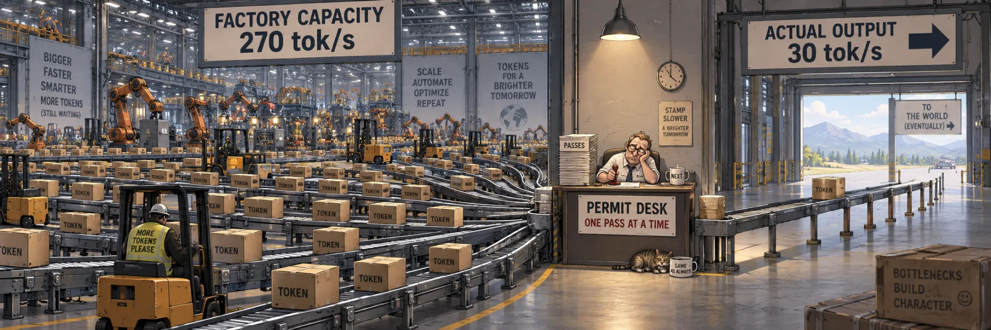
The fastest a language model can possibly write on a given card is something you can work out on paper, before running it.
Writing one token means running the whole network once, and running the network means every weight in it has to travel from the card's memory to the part of the chip that multiplies. Qwen2.5-0.5B holds 494 million of those weights, two bytes each — 0.92 GiB that must make the trip for every single token.
A Tesla T4 can read about 274 GB from its memory every second — measured on the card, not taken from its datasheet. At that speed, moving the model once takes 3.7 ms. No software can make a token arrive faster than its weights do, so this card and this model have a speed limit of 270 tokens a second.
The same model on the same card writes 30 tokens a second.
Where do the other 240 go?
It helps to know from the start that, at this level, almost every bottleneck in this note falls into one of three buckets:
- the bytes the card has to read from its memory,
- the arithmetic it has to do with those bytes,
- and how often it has to be told what to do next. A GPU runs programs called kernels — a kernel is a whole program, run by thousands of threads at once, and it is compiled and placed on the card ahead of time. What the host sends, over and over, is not the program but the order to run it: one command per operation, naming the kernel and the data. Between those commands the card does nothing on its own.
Almost everything below is one of those three becoming the limit at a different moment.
Answering the question properly takes the whole machinery of serving a language model — the loop that runs the model once per token, the two very different passes it is made of, the two waits a user feels, the weights that have to travel through memory at every step, and the way all of this changes when a card serves many people at once. This note goes through each of them from the hardware's side, measured end to end on one T4 with the half-billion-parameter model and a model three times larger for comparison. What happens inside the model — tokens, attention, sampling — is the subject of the generation note; here the model is a workload, and the question is what it does to the machine.
The generation loop
A serving process does not "run the model on a prompt". It runs a loop.
ids   ← tokenize(prompt)                      # CPU
cache ← allocate()                            # GPU memory for this request
next  ← model(ids, cache)                     # one pass over the whole prompt
while not finished:
    send(detokenize(next))                    # CPU → client
    next ← model(next, cache)                 # one pass over one token
Two properties of that loop decide almost everything that follows.
The first is that it is strictly sequential. The input of each iteration is the token the previous iteration produced: in ordinary autoregressive decoding, token cannot be finalized before token . A request's duration is therefore one pass over the prompt plus one pass per token of the answer, added up in a straight line.
The second is what stays on the GPU between iterations and what does not. The weights are loaded once and stay resident, but every iteration reads all of them again from memory. The cache — the keys and values that attention keeps for every earlier token, sized in its own short — stays resident too and grows by one token per iteration. What crosses between CPU and GPU per iteration is one integer: the token id. That is why streaming the answer to the client adds nothing measurable — the text is available the moment each iteration ends.
Here is one real request running through that loop: a 1,024-token prompt, a 32-token answer.
The GPU ran the model thirty-three times: once over the prompt, then once per token. The CPU's share was tokenizing — 3.8 ms to turn 5,130 characters into 1,024 ids — and detokenizing, 0.35 ms. Of the 1.28 seconds the request took, 0.3% was spent on anything other than running the model. Whatever makes inference slow or fast, it is not the text handling.
The loop itself is not free either, and it is worth knowing by how much. The same 32 tokens produced by a hand-written loop took 1,155 ms; produced by the library's own generate, 1,392 ms — the same tokens, bit for bit, 20% slower, because generate does bookkeeping around every iteration that a minimal loop skips. On a workload where each iteration is short, anything done once per iteration is expensive. That theme comes back.
Prefill: the prompt in one pass
The first iteration is special, and it has its own name: prefill.
All 1,024 prompt tokens are known before anything happens, so there is no reason to feed them in one at a time. They go through the model together, as a matrix of 1,024 rows. Attention's causal mask makes this equivalent to processing them one by one — each position still sees only the positions before it — so the result is identical and the work is done in a single pass.
That single pass does two jobs. It produces the first token of the answer, and it writes the cache: the keys and values of all 1,024 prompt tokens, 12 MiB for this model, which every later iteration will read.
As a workload for the GPU, prefill is the good kind. Multiplying a 1,024-row matrix by each weight matrix means every weight fetched from memory is used 1,024 times. Counted over the whole model, prefill performs 1,056 floating-point operations for every byte of weights it reads. On the roofline of this card the dividing line sits at about 76 operations per byte — below it a workload waits on memory, above it on arithmetic. Prefill is far above: it is compute-bound, the kind of work GPUs were built for.
Measured, prefill of 1,024 tokens took 137 ms and ran at 6.2 TFLOP/s. That is well below the 20.8 TFLOP/s this card sustains on its tensor cores, and where the time went says why. Attention accounts for only 4% of prefill's arithmetic — almost all of it is in the weight matrices — yet it took about two thirds of prefill's time: 39% on masking and softmax alone, 21% on the attention scores. Time does not follow arithmetic here. The weight multiplications run on the tensor cores at full efficiency; attention runs on a fallback path that is starved of bandwidth.
The fallback is a property of this particular combination of hardware, model and software, not of attention. PyTorch keeps several attention implementations behind one call, and for this model on a T4 with this version of PyTorch the fused ones all refuse: FlashAttention and the cuDNN kernel need a newer architecture, and the memory-efficient kernel will not broadcast this model's 2 key/value heads across its 14 query heads. What runs instead writes the entire score table — 1,024×1,024 numbers for every head — into memory, masks it, softmaxes it and reads it back. A fused kernel never writes that table out; keeping it inside the chip is the whole reason those kernels exist. The part of attention that compares every token with every earlier one also grows with the square of the prompt, which the section on the two waits measures directly.
Decode: the same weights, one row at a time
Every iteration after the first is a decode step: one token in, one token out, one more position appended to the cache.
It calls the same function on the same weights as prefill, but the input is a single row instead of 1,024. The weights that have to be read from memory are exactly the same. The arithmetic done with them is a thousand times smaller. Counted over the model, a decode step performs 1.1 floating-point operations per byte of weights — seventy times below the line where arithmetic becomes the limit. The matrix multiplication note shows why no kernel can improve that ratio: with one row there is no reuse of a weight to collect.
The trace of a real decode step (further down) shows the change at the level of kernels. With 1,024 rows, the weight multiplications run as matrix–matrix products on the tensor cores. With one row they run as matrix–vector products — a different family of kernels entirely, built for a job that is mostly reading.
So a decode step is best pictured not as a computation, but as a flow: the model's weights stream from memory, past the arithmetic units, once per token.
With one sequence decoding, the chip performs 1.1 operations on every byte it receives — about 1.5% of what it could do with that stream. Almost all of its arithmetic units spend the step waiting for the next weights to arrive.
The two waits: time to first token, time per output token
A user never sees prefill or decode. They see two waits: how long the screen stays empty, and how fast the text appears once it starts. Serving systems measure exactly those, under two names.
Time to first token (TTFT) is everything between sending the request and receiving the first token: network, time in the server's queue, tokenizing, and prefill. On this card, with nothing else queued, that was 3.8 ms of tokenizing plus 137 ms of prefill — 141 ms.
Time per output token (TPOT) is the gap between consecutive tokens once the answer is streaming: one decode step. Here it is 33 ms — 30 tokens a second, roughly four times faster than a person reads.
The total time of a request is TTFT plus the decode steps that follow, one per remaining token:
where the approximation holds as long as a step costs about the same at every point of the answer — true here, and not true once a growing context starts to cost something, which the section on the cache measures. That split is why the two are measured separately: they answer to different inputs and are fixed by different means. Holding the answer at a single token and stretching the prompt moves the first; holding the prompt and stretching the answer moves only the second.
Below 256 tokens the prompt is nearly free — 36 ms for 16 tokens, 37 ms for 256 — because a pass that small does not give the card enough work to be worth starting, and the time is the same fixed cost a single decode step pays. From 512 tokens prefill starts to cost what its arithmetic says, and then more: 151 ms at 1,024, 468 ms at 2,048, 7.2 seconds at 8,192. Eight times the prompt for forty-seven times the wait — the square-law part of attention, on a card where it runs the expensive way.
Stretching the answer instead leaves the first wait alone. Whether the answer is one token or five hundred, TTFT stays between 152 and 169 ms, while the request as a whole goes from 0.15 to 17 seconds.
So the two waits have two different owners. TTFT belongs to prefill: it grows with the prompt, and it depends heavily on how efficiently the hardware and software run attention. TPOT belongs to decode: in this regime it barely depends on the prompt — until the context gets long enough for attention and the cache to cost something of their own — and it depends above all on how fast the model's weights can be moved through the chip, which is the subject of the next section.
Model weights moving through memory
Since a decode step reads every weight once and does almost nothing else with them, its cost can be predicted from two numbers: the size of the model in bytes and the speed of memory.
The bandwidth in that formula was measured on this card by reading a large buffer: 274 GB/s, against 320 on its datasheet. For the 1.5-billion model, with 2.9 GiB of weights, the same arithmetic gives 11.4 ms.
This is the most important planning number in serving language models — once decode is actually limited by memory, model size divided by effective bandwidth is an excellent first-order predictor of its speed. It is why inference hardware is so often chosen by memory bandwidth rather than by arithmetic throughput, why storing weights in 8 or 4 bits instead of 16 is expected to speed decoding up in proportion, and why the speed of a large model running locally can be estimated from a laptop's memory bandwidth. The formula also runs the other way, on the denominator rather than the numerator: hardware that keeps the weights in memory on the chip itself, rather than in memory beside it, changes that figure by orders of magnitude rather than by percentages — which is where token rates far beyond anything a card like this can reach come from, and why such a rate is a claim about where the weights live before it is a claim about anything else. All of those predictions rest on one condition: that a decode step really is in that regime, limited by moving weights through memory and by nothing else first.
That condition is the thing to check, and a bound is not a measurement.
Which brings back the opening question. By this formula the small model should write 270 tokens a second. It writes 30.
Why decode is slow
A note on the numbers first, because several step times appear below and they are not the same measurement:
| step time | what was measured |
|---|---|
| 36.6 ms | mean decode step inside the one timed request — the first measurement after the model was loaded |
| 33 ms | the clean step: the median of consecutive steps at 1,024 tokens of context, before the profiler had ever run (32.7–33.8 ms across runs and context lengths) |
| 39.0 ms | the same step with the fixed-size cache a CUDA graph requires, launched one kernel at a time — the like-for-like baseline for the graph |
| 13.1 ms | that same step replayed as a CUDA graph |
| 39.0 / 40.0 ms | the clock check, rested and after a minute of work — measured late in the run, after profiling, so both carry the profiler's cost; what matters is that they agree |
The standard explanation is that decode is memory-bound: the memory cannot deliver the weights any faster. That is easy to test. A decode step moves 0.93 GiB in 33 ms, which is 31 GB/s. The memory can do 274. It is working at a ninth of its capacity.
So the memory is not the bottleneck — it is mostly idle, like the arithmetic units. Two more suspects need ruling out before looking at what the GPU is actually doing.
The card slowing itself down. GPUs lower their clock when they get hot or hit their power limit, and the GPU note showed this T4 doing exactly that. The same step was timed on a rested card and again after a minute of nonstop decoding: 39.0 ms and 40.0 ms (both measured after profiling, so both a little inflated — it is the comparison that counts), with the clock higher in the second case — 1,380 MHz against 1,200 — and the temperature unchanged. Not the clock.
The measurement itself. The natural next move is the profiler, which records every kernel the GPU runs. But attaching it makes every later kernel launch in the process a little more expensive, and it was measured here directly: the same step took 33.0 ms before the profiler had ever run and 39.5 ms after a single profiled call — 20% slower, for the rest of the process's life. Every timing in this note is taken before the profiler is switched on. And the size of that tax is a clue in itself: a tool that adds cost per launch slows a workload by a fifth only if the workload is mostly launches.
Here is what the profiler sees: a real trace of one decode step, the CPU handing out work in the top lane, the GPU doing it in the bottom one.
One decode step of this model is 1,414 separate kernel launches — 1,414 times the host says "run this one now", for programs that are already sitting on the card. The model is called once from Python; the individual kernels are launched underneath, by PyTorch's eager execution path through its dispatcher and the CUDA runtime, one operation at a time. The typical kernel runs for 3.4 µs. The typical gap before the next one starts is 24.9 µs. The trace is taken under the profiler, which widens every gap, but the clean numbers say the same thing: the kernels of a step are busy for about 10 ms of its 33. The GPU finishes each small piece of work almost instantly and then waits for the host to submit the next one.
A second measurement shows it without the profiler at all. Time each stage of the model on its own and add up a step's worth: the twenty-four normalizations — a few thousand parameters each, no matrix multiplication between them — take 4.0 ms, almost as much as the entire MLP, which holds 64% of the model's weights (4.9 ms). At batch 1 a stage costs what it costs because it is a kernel launch, not because of what it computes.
The diagnosis is testable. A CUDA graph records the whole sequence of kernels once and replays it as a single submission: same kernels, same arithmetic, same bytes, only the per-kernel handover removed. Switch the trace to the graph and the gaps close — one launch call instead of 1,414, the typical gap down from 24.9 µs to 0.4 µs, the GPU busy for 96% of the step instead of 19%. Timed cleanly, with the fixed-size cache a graph requires, the step goes from 39.0 ms launched one kernel at a time to 13.1 ms replayed as a graph.
So decode on this setup is not memory-bound. It is launch-bound: most of the time goes on the host-side cost of dispatching and launching work in eager execution, not on doing it. The memory wall is real, but it stands behind this one, and it comes into view as the model grows. The 1.5-billion model needs 11.4 ms of memory traffic per token; replayed as a graph it takes 25.9 ms and moves 120 GB/s — nearly half the card's bandwidth, against the small model's 77. The heavier the weights, the larger the share of each step spent actually reading them, and the closer a system comes to the regime the textbook describes.
That is why inference engines capture graphs, fuse kernels and compile models before doing anything else. On small models and at small batch sizes, that work is not a micro-optimization; it is most of the time on the table.
What grows: the cache
The weights are a fixed cost, paid in full at every step and the same for every request. The cache is the part that grows: every token adds its keys and values, 12 KiB here, and every later step reads them.
At this scale the growth is almost invisible in the time. From 128 tokens of context to 8,192 — sixty-four times more — the small model's step goes from 33.5 to 34.4 ms: its cache grew from 1.5 MiB to 96 MiB, against 942 MiB of weights re-read at every step regardless, and all of it hidden behind the launch cost. A thousand tokens generated one after another say the same from the other side: the last thirty-two cost what the first thirty-two cost. The larger model is flat as well until 8,192 tokens, where its step jumps from 44 to 71 ms — more than its 224 MiB of cache can account for by bytes, and the square-law attention again.
Where the cache does bite is memory capacity, because it is the one thing that is not shared.
The weights are loaded once and serve every conversation on the card. The cache belongs to one conversation and grows with every token in it: 12 KiB per token for the small model, 28 KiB for the larger one. At 32,768 tokens of context the larger model's single conversation carries 896 MiB — a third of the model itself, for one user. The weights decide whether a model fits on a card at all. After that, capacity is counted in conversations times their length.
Latency and throughput
Everything so far has been one request alone on the card. A real server has many, and that introduces the distinction that runs through all of serving.
Latency is what one user experiences: the TTFT and TPOT of their request. Throughput is what the machine produces: tokens per second across every request it is serving. They sound like two views of one number. They are not, and the reason is the stream of weights.
If a decode step is the whole model streaming past the chip, a second sequence initially costs almost nothing: it rides on the same stream, getting its own multiply-add per weight from bytes that were being read anyway. Go back to the flow widget above and move the slider. Up to 16 sequences the step stays at 33–36 ms — every one of those sixteen users still gets a token about every 36 ms — while the machine goes from 30 tokens a second to 445. Throughput rises fifteenfold; latency barely moves. That is batching, and it is the single most important economic fact about serving language models.
The roofline says how long it should last. At 16 sequences the chip does about 15 operations per byte; every sequence also brings its own cache to read, so the ratio climbs more slowly than the batch, and at this 512-token context it would reach the card's 76 at around 146 sequences. The free ride should end there.
It ends long before. At 32 sequences the step jumps to 55 ms, at 64 to 100 ms; each user's rate collapses from 30 tokens a second to 10, while the machine's total barely improves, from 582 to 637. Between 16 and 64 sequences throughput rises by 43% and latency triples.
The trace shows why, and it vindicates the roofline where the roofline applies. At 64 sequences the multiplications by the weights take 6.9 ms of the step — hardly more than at 16. The weights really are shared, just as the physics says. What grew is everything that is not shared: each sequence's cache being copied and rearranged every step (37 ms), and attention's own arithmetic, which on this card runs in 32-bit precision through the fallback path (about 50 ms between its element-wise work and its own matrix–vector products). Of 96 ms of GPU work at batch 64, the weights are seven.
That is the shape of batching on any hardware: the weights amortize, the per-sequence work does not, and the free ride ends wherever the per-sequence work takes over. How early that happens depends on how efficiently a system handles the cache and attention — here, on an old card without fused attention, it happens at 32.
Which point on that curve to sit at is a policy, not a technical fact. A service that promises fast replies keeps batches small and pays for more cards; a service that processes documents overnight packs the card full and accepts slow individual answers. Both are running the same model on the same hardware.
A last honest limit: these are static batches, formed and run together. Real requests arrive at different moments, bring prompts of different lengths and finish at different points, and a real server has to decide what to admit while work is already in flight. That is a harder problem than the one measured here.
So why not just optimise it?
The honest reply to the gap is to close it and see how far that gets. Four rungs, same card, same two models, all at batch 1 with 1,024 tokens of context — measured in their own session, which is why the graph rung reads 12.3 ms here against the 13.1 ms above: the same measurement, a different run:
| 0.5B model | 1.5B model | |
|---|---|---|
| plain PyTorch, as measured above | 33.2 ms · 30 tok/s | 37.6 ms · 27 tok/s |
| the step replayed as a CUDA graph | 12.3 ms · 82 tok/s | 21.3 ms · 47 tok/s |
torch.compile, reduce-overhead | 13.1 ms · 77 tok/s | 19.1 ms · 52 tok/s |
| vLLM, an engine built for this | 6.1 ms · 164 tok/s | 16.6 ms · 60 tok/s |
| the floor from bytes | 3.7 ms · 273 tok/s | 11.4 ms · 88 tok/s |
Each rung removes something different. The graph removes the per-launch handover and nothing else — same kernels, same order. Compilation removes launches too, and fuses neighbouring operations on the way, which is why on the larger model it beats the hand-made graph (19.1 ms against 21.3) while on the small one the two land together. The engine does all of that and replaces the kernels as well: on this card it runs attention through a Triton kernel instead of the fallback path, and it keeps its own cache in fixed blocks so nothing is copied between steps.
The result is that most of the gap really does close. The small model goes from nine times its floor to 1.7 times, and from 11% of the card's memory bandwidth to 60%. The larger model ends at 1.5 times its floor and 69% of bandwidth — a model with three times the weights was always closer to the wall, and after optimisation there is almost nothing left between it and the bytes.
The same applies to the other wait. With a 2,407-token prefix shared between requests — a system prompt, a document everyone asks about — the engine can reuse the cache of that prefix instead of computing it again: 505 ms of TTFT becomes 47 ms, ten times less, for the price of the first request paying in full.
None of this is free, which is the other half of the answer. Graphs and compilation need shapes that never change, so the cache has to be allocated for the longest answer the request might produce, whether it produces it or not. Compiling cost about 30 seconds of start-up per model here. An engine takes over the loop, so anything custom inside it — an unusual sampler, a per-request adapter — is now its business rather than yours. And the numbers above are batch 1; a system that serves many users at once is buying throughput, which is a different budget.
What does not move is the last factor of 1.5. That part is the weights themselves: every token reads them once, and the only ways past it are fewer bytes per weight or more tokens per read — quantisation or batching, not better scheduling.
What a production inference engine changes
The engine above wins by doing several things at once, and it is worth separating them, because each is aimed at a different wall. Two of them are already measured here — graph capture and compilation against the launch-bound step, prefix reuse against time to first token — and the rest are the reason a serving stack is more than a fast forward pass.
Fused attention kernels attack the prefill fallback. They compute attention without ever writing the score table to memory, and on hardware and model shapes they support, attention's share of prefill falls from the majority to a small part. The engine used one on this card, which is part of why its decode step is half of the hand-made graph's.
Continuous batching attacks the limit of static batches. Instead of forming a batch and running it to the end, the engine adds and removes sequences at every step, so a finished request frees its place immediately and a new one joins without waiting for the rest.
Paging the cache attacks memory capacity. The cache is allocated in small fixed-size blocks as a conversation actually grows, instead of being reserved up front for the longest possible answer, so memory holds the conversations that exist rather than the ones that might.
Quantization attacks the bytes floor. Fewer bytes per weight lower the 3.7 ms bound in proportion — and pay off in proportion only once the step is really limited by those bytes, which is exactly the condition this note checks.
Splitting a model across GPUs attacks the case where one card's memory or bandwidth is not enough: each card holds and streams a slice of every weight matrix, their bandwidths add up, and the price is communication between the cards at every step.
Each of them is aimed at one of the three limits from the start of this note — bytes, arithmetic, or the work handed to the GPU.
Back to 270 and 30
The opening question has an answer now, and it is spread across every part of the machine this note went through.
The 270 tokens a second was a prediction about moving weights through memory, and it describes decode correctly as physics: one row of input, 1.1 operations per byte, every weight read at every step. What it leaves out is everything around that transfer. On this card and this model, most of a decode step was the GPU waiting between 1,414 small kernels — which is why the same work, replayed as one graph, runs at 13.1 ms instead of 39, and why an engine that also brings its own kernels and cache gets a token in 6.1 ms, 164 a second, at 60% of the card's memory bandwidth.
So the 30 was never a fact about the hardware; it was a fact about how the model was being run. The 270 is not reachable either, because it assumes perfect use of memory and nothing else happening — but 164 is, and what separates it from 273 is no longer software. It is the weights themselves, read once per token, which only fewer bytes or more tokens per read can change.
There is a general shape in that, and it is worth saying plainly: optimising does not remove limits, it moves which one is binding. On this card the step began limited by how often the GPU had to be told what to do; take that away with graphs and compilation and it becomes limited by the kernels; replace those too and it becomes limited by the bytes. Each rung ends at a wall that the previous rung was hiding — and the wall at the end is not a flaw in anyone's software. It is what the hardware is.
Past that point improvements are no longer free; they are trades. Fewer bytes per weight buys speed and pays in accuracy. A larger batch buys throughput and pays in the latency of everyone in it. A smaller model buys everything and pays in what it knows. More cards buy bandwidth and pay in money and in communication at every step. Which of those is worth making is a question about the service, not about the GPU — but knowing which wall is currently binding is what makes the question answerable at all, and that is what a floor, a clean measurement and a trace are for.
The same map explains the rest. The wait before the first token belongs to prefill and grows with the prompt, faster than linearly where attention runs without a fused kernel. The pace after it belongs to decode and barely depends on the prompt until the context grows long. Extra sequences ride on the same stream of weights for free until what each of them brings along — its cache, its share of attention — outweighs what they share. And memory fills up with conversations long before it fills up with the model.
Four numbers carry most of it: 3.7 ms from arithmetic, 33 ms from a clean measurement of the plain stack, 13.1 ms once the launches are gone, and 6.1 ms from an engine built to keep the card busy. The first says what the hardware allows, the second what a system actually did, and the last two how much of the difference was never the hardware's to begin with.