Training Neural Networks: Backprop, Regularization, and Everything in Between

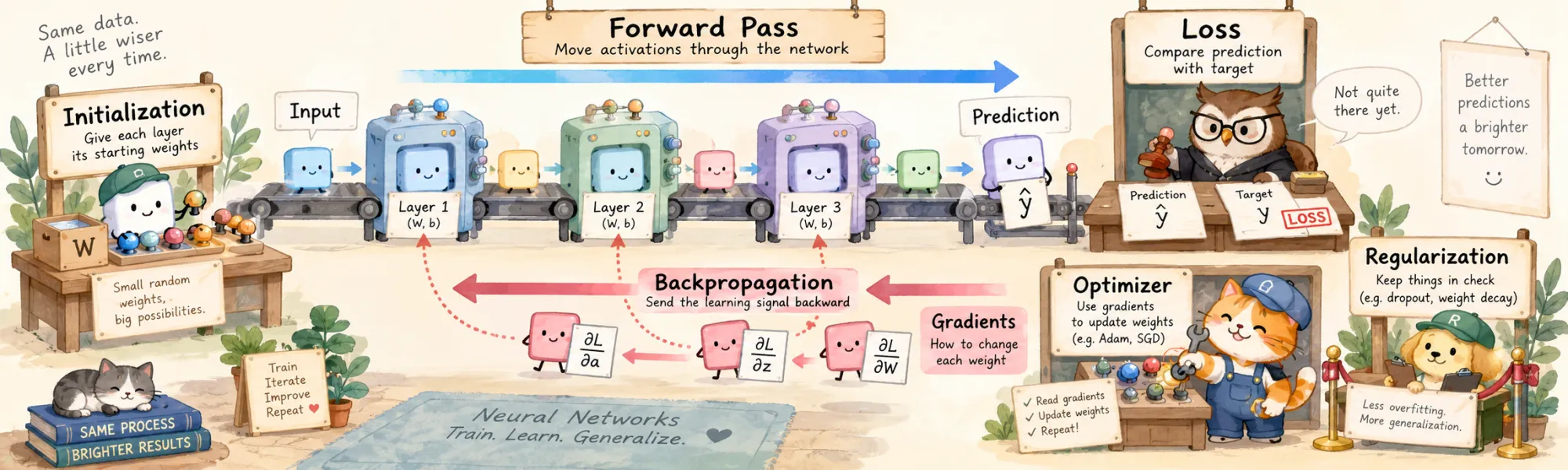
A trained network is a pile of numbers that happens to be useful. Training is the process that made them useful, and it is far more mechanical than the word learning suggests. The network produces an answer. We measure how wrong that answer is, as a single number. And then that single number has to become an instruction for every adjustable number inside the network: this one up, that one down, and by how much.

That trip — from one scalar at the end to millions of instructions inside — is the entire subject. Backpropagation is the algorithm that makes it. Initialization and normalization are the conditions under which the instruction survives the journey instead of dying or exploding on the way. Regularization is the set of constraints, perturbations and training choices that push the result towards generalizing instead of memorizing. They look like unrelated topics; they are parts of one story, and reading them as one is the point of this note.

Two threads run through all of it, worth naming before we start.

The first is a product of many numbers. A gradient that has travelled back through $L$ layers is a product of $L$ factors. In the scalar toy model below those factors are plain numbers; in a real network they are Jacobian matrices, so some directions can shrink while others grow at the same time — but the multiplication problem survives the upgrade intact. If those factors are typically a little below one, the product vanishes exponentially; a little above one, it explodes exponentially. Vanishing and exploding gradients are that fact directly, and initialization schemes and residual connections are built around it.

That product sits inside a broader problem, which is the one the note is really about: for training to work, the signal that reaches a parameter has to be informative — it has to say something true about that parameter's effect on the loss — it has to stay numerically representable on the way, and it has to arrive at all. Different techniques attack different parts of that, and it is worth resisting the temptation to collapse them into one slogan. Normalization keeps each layer's inputs in a range where the optimization behaves. Gradient clipping repairs no product; it bounds the step once the gradient already exists. bf16 stabilizes nothing either — it widens the range of numbers you can write down. Cross-entropy changes the very first factor in the chain rather than any of the later ones. One problem, several faces.

The second is blame is local. To compute how the final loss depends on some weight buried deep inside, that weight does not need to know anything about the network. It needs its own local derivative and the error signal handed to it from above — one number in the scalar chain, a vector in a real layer — and where its output feeds several places downstream, the signals coming back along each path are simply added up. Nothing else. That is why automatic differentiation libraries exist, why a network of nearly arbitrary shape can be trained without anyone deriving a single formula by hand, and why all the gradients together cost a small constant multiple of one forward pass rather than one forward pass per parameter.

Nothing here is taken on faith. Every claim that matters is pinned to a small experiment with real numbers, run for this note — a widget to poke at on the page, and the whole thing end to end in the companion lab. In three places the measurement disagreed with the tidy version of the story, and in those places what you get is the measurement.

One chain of reasoning runs through the whole note, and it is worth saying up front what it is, because it will keep coming back. We start with a network so small it can be computed by hand: two weights, one input, one number out. We work the entire training step on it — forward, loss, backward, update — with real arithmetic, no notation left standing on its own. Then we take that same chain and stretch it: the same two multiplications become twenty, and every difficulty of deep learning appears immediately, in a model still small enough to reason about completely. Then we widen it into a real network on real data, where the same quantities stop being computed by hand and start being measured. Same chain, three magnifications. The experiments behind them necessarily run on different data — four points, a few thousand digits, two hundred digits — but the object under the microscope is the same one throughout.

---

Before backprop: a learning rule that only worked for one layer

Start with why this was hard, because the shape of the difficulty explains the shape of the solution.

The perceptron (1958) is a single artificial neuron: it takes inputs, weights them, sums, and fires if the sum clears a threshold —

$$\hat{y} = \text{step}(w \cdot x + b).$$

It came with a learning rule that is charmingly direct. Show it an example. If it gets the answer right, change nothing. If it gets the answer wrong, nudge every weight in the direction that would have helped:

$$w \leftarrow w + \eta\,(y - \hat{y})\,x.$$

That rule has a real theorem behind it: if the data can be separated by a straight line, the perceptron finds such a line in a finite number of steps. Guaranteed.

The trouble is the if. The standard demonstration is XOR, four points and two classes: $(0,0) \to 0$, $(1,1) \to 0$, $(0,1) \to 1$, $(1,0) \to 1$. Draw the four points on paper and try to separate the two classes with one straight line. There is no such line — the two positive points sit on opposite corners. The perceptron does not fail to find a good line here; it fails because no line exists. Run the rule anyway and it never settles: it falls into a cycle, each fix breaking a point the previous fix had repaired.

This is what the 1969 critique made precise, and it helped cool enthusiasm for perceptron-style learning for years afterwards — one cause among several, not the single switch that turned a field off. But the interesting part is not the failure — everyone already knew a stack of neurons could carve XOR out of the plane with two lines. The interesting part is why nobody could train the stack.

The perceptron rule needs $(y - \hat{y})$: the difference between what the unit produced and what it should have produced. For the output unit, we have that. For a unit in the middle, we do not. Nobody knows what the hidden unit should have produced. There is no target for it. The data says what the network should output; it says nothing whatsoever about what any intermediate value should be.

That is the actual blocker, and it is worth stating in one line, because backpropagation is precisely its answer:

Backpropagation manufactures an error signal for units that have no target of their own.

It does that by asking a question the perceptron rule never asks — not "what should this unit have produced?", but "if this unit's output had been slightly different, how would the final loss have changed?" That second question has an answer even for a unit buried five layers deep, and the answer is computable. That change of question is the whole idea. Everything below is machinery for answering it efficiently.

Run on those four points, the perceptron rule does not thrash — it settles into a loop. After an early peak at 75% the weights at the end of every epoch become identical to the epoch before, and accuracy sits at 25%, worse than guessing. Nothing is broken; the rule is doing exactly what it promises, and what it promises is unreachable here. Give it a problem a line can solve — AND instead of XOR, same four points, same code — and it converges to 100% in six epochs.

A 2-2-1 network trained by backprop solves XOR in 24 to 46 epochs on four of five random starts. On the fifth it does not solve it at all within 600, which is worth reporting rather than averaging away: two hidden units is a tight budget, and where the weights happen to start decides whether the net finds the solution. That is the initialization section, arriving early and uninvited.

---

The example: two weights, computed by hand

Here is the network we will be living with. It has one input, one intermediate value, one output, and exactly two adjustable numbers:

$$x \;\longrightarrow\; \times\,w_1 \;\longrightarrow\; h \;\longrightarrow\; \times\,w_2 \;\longrightarrow\; \hat{y} \;\longrightarrow\; L$$

Written out, the whole model is two multiplications and a loss:

$$h = x\,w_1, \qquad \hat{y} = h\,w_2, \qquad L = (\hat{y} - y)^2.$$

No layers to speak of, no nonlinearity yet, nothing to hide behind. Give it numbers. The input is $x = 2$. The weights currently sit at $w_1 = 3$ and $w_2 = 4$ — they are wherever initialization put them, and there is nothing special about these values. The correct answer for this input is $y = 20$.

Run it forward. The intermediate value is $h = 2 \times 3 = 6$. The prediction is $\hat{y} = 6 \times 4 = 24$. We wanted 20, so the loss is $L = (24 - 20)^2 = 16$.

Notice what the forward pass has and has not told us. It has told us exactly what happened: 2 became 6, 6 became 24, and that prediction cost us 16. It has not told us what to do. We have one number at the end — 16 — and two knobs inside, and no instruction for either of them. Should $w_1$ go up or down? By how much? What about $w_2$? Squaring the error made it a clean positive number, but a positive number alone points nowhere.

The expensive answer. There is an obvious way to find out. Take $w_1$, nudge it by some tiny $\varepsilon$, run the entire network forward again, and see which way the loss moved. Then put $w_1$ back, do the same for $w_2$. With two weights this is mildly annoying. The arithmetic of doing it at scale is what kills it: the cost is one full forward pass per parameter, per update. A model with a hundred million parameters would need a hundred million forward passes to decide on a single step, and then another hundred million for the step after that.

A network with a hundred million parameters, built and timed on a CPU for this note, takes 18 ms for one forward pass. Nudging each parameter once would therefore take about 500 hours of forward passes — three weeks — to decide on a single update, and then start over for the next one.

That is not a rounding-error inefficiency, it is the difference between a method that exists and one that does not. What we want instead is all the gradients from something that costs a small constant multiple of one forward pass. That is what backpropagation delivers, and it delivers it with nothing more exotic than the chain rule.

---

Backpropagation: the chain rule, run backwards

The trick starts at the end, because the end is the only place where we know anything for certain: we know the loss, and we know the prediction that produced it.

Step one — how does the loss respond to the prediction? The loss is $L = (\hat{y} - y)^2$, so

$$\frac{\partial L}{\partial \hat{y}} = 2(\hat{y} - y) = 2(24 - 20) = 8.$$

In plain terms: if the prediction crept up by a hair, the loss would rise about eight times as fast as that hair is thick. Positive, so pushing the prediction higher makes things worse; we want it lower. This is the only place in the whole procedure where the loss function itself appears. Everything after this is the network.

Step two — how does the prediction respond to $w_2$? The prediction is $\hat{y} = h\,w_2$, and right now $h = 6$. Multiplication is easy to differentiate: nudge $w_2$ by a hair, and $\hat{y}$ moves six times as much, because it gets multiplied by 6 on the way out. So $\partial \hat{y} / \partial w_2 = h = 6$.

Now chain the two together. Changing $w_2$ changes $\hat{y}$, and changing $\hat{y}$ changes $L$, so the effect of $w_2$ on $L$ is the product of the two:

$$\frac{\partial L}{\partial w_2} = \frac{\partial L}{\partial \hat{y}} \cdot \frac{\partial \hat{y}}{\partial w_2} = 8 \times 6 = 48.$$

That is a real instruction at last. It is positive, so increasing $w_2$ increases the loss; to reduce the loss, $w_2$ must come down.

Step three — carry the signal one step further back. Now $w_1$, which is further from the loss: it changes $h$, which changes $\hat{y}$, which changes $L$. We could grind out that whole chain from scratch, but we already own most of it. We know the loss responds to $\hat{y}$ with a factor of 8. So we only need one new local fact: how $\hat{y}$ responds to $h$. Since $\hat{y} = h\,w_2$ and $w_2 = 4$, a hair of change in $h$ produces four times as much change in $\hat{y}$. Therefore

$$\frac{\partial L}{\partial h} = \frac{\partial L}{\partial \hat{y}} \cdot \frac{\partial \hat{y}}{\partial h} = 8 \times 4 = 32.$$

We have just taken information about the final loss and moved it one station back along the network. That number, 32, is the "error signal" for $h$ — the target the perceptron rule could never supply. Nobody said what $h$ should have been. We instead know how sensitive the final loss is to $h$, and it turns out that is all we ever needed.

Step four — and now $w_1$ is easy. $h = x\,w_1$ with $x = 2$, so nudging $w_1$ moves $h$ twice as much:

$$\frac{\partial L}{\partial w_1} = \frac{\partial L}{\partial h} \cdot \frac{\partial h}{\partial w_1} = 32 \times 2 = 64.$$

Both gradients, done:

$$\frac{\partial L}{\partial w_1} = 64, \qquad \frac{\partial L}{\partial w_2} = 48.$$

Look at what that cost. We never perturbed a weight and reran the model. We started at the loss, computed one local derivative, used it to step back, then reused that result to step back again. Each station along the way needed exactly two things: its own local derivative, which is trivial arithmetic, and the number handed to it from the station above. That is the second thread — blame is local — and it is why this scales. Adding a third weight would not have made the first two any more expensive to compute; it would have added one more step to the same walk backwards.

The one pattern worth memorizing. Look at $\partial L / \partial w_2 = 8 \times 6$ and $\partial L / \partial w_1 = 32 \times 2$. Both have the same shape: what came back from above times what came in from below. In a linear layer, the gradient for a weight is the incoming activation multiplied by the error signal arriving at that weight's output — a rule for that shape of operation, not a universal law, since every operation has its own local derivative and that is exactly what the framework stores. When this generalizes to a real layer $y = Wx + b$, with $\delta = \partial L / \partial y$ the error arriving at the layer's output, it becomes

$$\frac{\partial L}{\partial W} = \delta\, x^{\top}, \qquad \frac{\partial L}{\partial b} = \delta, \qquad \frac{\partial L}{\partial x} = W^{\top} \delta.$$

Three lines, and they are the entire backward pass of a fully-connected layer. The last one is worth staring at: to send the error further back, you multiply by the transpose of the same weight matrix the forward pass used. The backward pass runs the same numbers through the same matrix in the other direction. There is no second network holding backward weights; there is one set of weights, read forwards to predict and read sideways to assign blame.

The update, and who does it

Backpropagation has now done its entire job. Notice what it has not done: it has not changed a single weight. It produced two numbers, 64 and 48, and stopped. Turning gradients into new weights is a separate job with a separate name — the optimizer — and keeping the two apart avoids a great deal of confusion later.

The simplest optimizer takes a small step against the gradient:

$$w \leftarrow w - \eta\,\frac{\partial L}{\partial w}.$$

The gradient points uphill on the loss; we want down, hence the minus. And we take a small step, scaled by the learning rate $\eta$, because the gradient describes the slope right here and says nothing about the terrain further along. With $\eta = 0.01$:

$$w_1 = 3 - 0.01 \times 64 = 2.36, \qquad w_2 = 4 - 0.01 \times 48 = 3.52.$$

Run the network forward again with the new weights. $h = 2 \times 2.36 = 4.72$. $\hat{y} = 4.72 \times 3.52 \approx 16.61$. The loss is $(16.61 - 20)^2 \approx 11.5$, down from 16.

One step, and it worked. And notice what the model was never told: nobody informed it that $w_1 w_2 = 5$ would be perfect. It knew how wrong it was and what the local slope looked like, and that was enough to move in a useful direction. Repeat that a few thousand times and the process has a name that sounds like understanding.

Why frameworks do this and you do not

The steps above generalize mechanically, which is exactly why nobody performs them by hand. A framework records the operations of the forward pass as a graph — every node knowing its inputs and its own local derivative rule — and then walks that graph backwards, multiplying and accumulating. That is what happens inside .backward(), and the architectures note treats the machinery as one of PyTorch's three core ideas.

Two consequences are worth carrying around.

The backward pass costs a small constant multiple of the forward pass. Reverse-mode differentiation computes every parameter's gradient in one backward sweep, and each node does a bit more arithmetic going back than it did coming forward — on the dense networks measured below, the backward pass alone costs about 1.4 to 2.0 forward passes, so forward and backward together cost roughly 2.4 to 3.0. Not a hundred million times it. That constant factor, instead of one forward pass per parameter, is the single fact that makes deep learning possible, and it comes from the reuse we saw in step three: $\partial L / \partial h$ was computed once and served every parameter below it.

The price is memory. To compute $\partial L / \partial w_2 = 8 \times 6$ we needed $h = 6$ — a value from the forward pass, still sitting around when the backward pass came looking for it. The forward values the backward pass needs have to stay available until their gradients are computed. That is one reason training costs more memory than inference, though it is worth being exact about the size of it: on the networks measured below the activations were the smaller half of the bill. The dependable multiplier is the optimizer — gradients plus Adam's two moment estimates are three extra copies of every parameter, held for the whole run. Activations are the part that grows with batch size and depth, and the standard escape hatch, gradient checkpointing, trades against exactly them: throw them away and recompute during the backward pass, paying time to save space.

There is also a reason this runs backwards rather than forwards. Derivatives can be propagated in either direction. Going forwards, you pick one input and compute how everything downstream responds to it — one sweep per input. Going backwards, you pick one output and compute how it responds to everything upstream — one sweep per output. Training has millions of inputs to the derivative (the parameters) and exactly one output (the scalar loss). The direction that costs one sweep per output is the obvious winner, and it is not a close call.

Across four network sizes the backward pass alone costs 1.4 to 2.0 times the forward pass, so the gradient for every parameter — forward and backward together — arrives for 2.4 to 3.0 forward passes, and 3.6 on the hundred-million-parameter network. That price still grows with the network, since a bigger network is a bigger forward pass; what does not grow is the number of sweeps, which stays at one backward pass however many parameters there are. One-sided finite differences on the same networks cost 7,300× a forward-and-backward step at 26 thousand parameters and 2.1 million× at 6 million. Put in wall-clock: for the 6-million-parameter net, one finite-difference gradient is 4.6 hours; backpropagation returns the same thing in 8 milliseconds. (Central differences, the more accurate kind used to check gradients, need two forward passes per parameter and double every one of those figures.)

The memory column is the less dramatic half. At batch 128 the tensors autograd kept for the backward pass came to 3.6 MB against 24.2 MB of parameters — saved activations grow with batch and depth while parameters do not, so the ratio flips for large batches and long sequences, but on this shape they were not the dominant cost.

---

The product of many numbers

Now stretch the example. Same chain, same idea, only longer: instead of two multiplications, twenty. Each layer is one weight, and the network is

$$\hat{y} = x\,w_1 w_2 \cdots w_{20}.$$

Run the backward walk on this and something jumps out. The gradient for the first weight is

$$\frac{\partial L}{\partial w_1} = \frac{\partial L}{\partial \hat{y}} \cdot x \cdot (w_2 w_3 \cdots w_{20}).$$

The instruction reaching the earliest weight has been multiplied by every weight that comes after it. Nineteen factors, all multiplied together.

That is the first thread in its plainest form, and the consequences are not subtle. Suppose every weight happens to be around $0.5$. Then that product is $0.5^{19} \approx 2 \times 10^{-6}$: the first layer receives an instruction two million times fainter than the last layer's. It is not being told to stay still — it is being told something, in a whisper below the noise floor of the arithmetic. Now suppose every weight is around $1.5$ instead. The product is $1.5^{19} \approx 2200$, and the first layer receives an instruction so violent that a single step throws it somewhere random.

Nothing about this needs a real network to appear. It is twenty numbers multiplied together, and the outcome is exponential in the depth either way. Deep networks are, from the gradient's point of view, exactly this: a long product, with all the numerical tact that implies.

Where the factors actually come from. In a real network each link contributes two things rather than one — the weight, and the derivative of the activation function at that point. The chain link is $w \cdot \sigma'(z)$, and the activation's derivative turns out to be the historically decisive half.

Take the sigmoid, the standard choice for decades. Its derivative peaks at $0.25$, dead centre, and falls towards zero in both directions. The layer's full contribution to the chain is its weights and that derivative, so the sigmoid does not set the whole factor by itself — but it caps its own share of it at a quarter, and usually contributes far less than that, since a unit sitting away from centre has a derivative smaller by orders of magnitude. Stack ten such layers and the activations alone contribute at most $0.25^{10} \approx 10^{-6}$, best case. This is not a tuning problem; it is a ceiling built into the function, and it is one major reason deep sigmoid feed-forward networks were notoriously difficult to optimize.

ReLU removes the ceiling by the simplest possible means: $\max(0, x)$ has derivative exactly $1$ wherever it is active. Not $0.9$, not $0.25$ — one. A gradient passing through the activation of an active ReLU is not damped by the activation at all. The price is that an inactive unit passes nothing — at initialization, with a symmetric zero-mean input, that is roughly half the units — which is a real cost but a different kind of cost: some paths are cut, rather than every path being attenuated.

Residual connections attack the same product from the other side. Wire a layer as $y = x + f(x)$ and its local derivative is $1 + f'(x)$ — that $1$ is an undamped path straight through, so the gradient reaching the bottom is no longer a bare product of small factors. For a real layer the scalar becomes a matrix, $I + J_f$, and the intuition survives the upgrade with one qualification worth keeping: the identity term gives the gradient a direct path around every block, but it guarantees nothing about the total. The two contributions add, and depending on $J_f$ the sum can come out larger than the signal that arrived — or, in some directions, smaller. This is the same structural trick as the LSTM's cell state, discovered twice for the same reason, and it is why networks jumped from tens of layers to hundreds.

Forty layers, one backward pass on a real MNIST batch, gradient norm at every layer. With ReLU and He the profile is flat: 0.70 at the second layer against 1.10 at the top. Forty layers, and the signal arrives intact. Swap only the activation for a sigmoid: the top still sees 0.47, the bottom sees 5 × 10⁻²⁰. Nineteen orders of magnitude lost on the way down, and no learning rate reaches across that.

Then the factor of two, which is easy to dismiss as a detail. Initialize the same ReLU stack with the forward-only $1/d_\text{in}$ instead of He's $2/d_\text{in}$, and the gradient at the bottom is 5 × 10⁻⁷ — 1.3 million times smaller than the He run. The arithmetic predicts it before the experiment: ReLU costs a factor of 2 in variance per layer, so forty layers should cost about $2^{20} \approx 1.05$ million, and the measurement lands within 25% of that. One constant, compounded twenty times.

Residual connections, measured here without normalization, do precisely what the qualification above warned they would. The gradient no longer vanishes — it reaches 7 × 10⁸. Adding $x$ to $f(x)$ also adds their variances — exactly so when the two are roughly uncorrelated, as they are here at initialization — so the direct path is undamped in both directions: it lets the signal through and says nothing about the size it arrives at. That is why residual stacks are typically paired with a normalization layer. Normalization-free designs exist, but they get there with careful initialization and scaling of their own; normalization is where the note goes after initialization.

The architectures note measures the mirror image of this — whether the signal survives the trip forward through forty layers. Same forty layers, same three initialization scales, opposite direction. Worth holding both pictures: a network can be broken on the way in, on the way out, or both, and the fixes are the same fixes because it is the same product.

---

Initialization: one constant decides whether it trains at all

The long chain also tells us, without any further theory, what the weights ought to look like at the start. We need the product of many factors to stay near one. In the scalar chain — and only in the scalar chain — that is a one-line answer: the typical magnitude of $w$ should be about $1$. Below and the gradient dies with depth, above and it detonates.

A real layer is the same statement with bookkeeping. A unit sums $d_\text{in}$ weighted inputs, and summing independent random terms adds their variances, so the output variance is $d_\text{in}$ times the variance of a single product. To keep the forward scale from growing layer to layer we need that to come out to roughly one, which gives

$$\text{Var}(W) = \frac{1}{d_{\text{in}}}.$$

A unit with 1000 inputs must start with weights about $\sqrt{1000} \approx 32$ times smaller than a unit with one input, or its output is 32 times too loud before training even begins.

That is only half the argument, though, and the half that gets quoted. The backward pass has its own claim on the same matrix: the gradient travels back through $W^{\top}$, so running the identical variance bookkeeping in the other direction asks for $\text{Var}(W) = 1/d_{\text{out}}$. Two conditions, one matrix, and they disagree in every layer that changes width. Glorot initialization — the one usually called Xavier — is the compromise between them:

$$\text{Var}(W) = \frac{2}{d_{\text{in}} + d_{\text{out}}},$$

which is one over the average of the two fan counts, and collapses back to $1/d_{\text{in}}$ exactly when the layer is square. Worth knowing which is which: the widely-repeated "one over fan-in" rule is the forward-only condition, not Glorot's, and the difference only bites where a layer's width changes sharply.

He initialization re-runs the argument for ReLU:

$$\text{Var}(W) = \frac{2}{d_{\text{in}}}.$$

The factor of two is not a fudge. For a symmetric, zero-mean input, ReLU zeroes about half the units, so roughly half of the second moment survives the activation, and doubling the variance going in compensates. Only roughly: ReLU's output has a non-zero mean, so its variance is not literally halved, and the derivation leans on assumptions about the input distribution that hold at initialization and drift afterwards. Two schemes, one idea, a constant of difference — and the constant matters, because it is raised to the power of the depth.

And zero is a special kind of wrong. Initializing all weights to zero seems safe and is catastrophic, for a reason that has nothing to do with scale. If every unit in a layer starts identical, every unit computes the same output, and — walking the backward pass — every unit receives the same gradient. So they all update identically and stay identical. Forever. A thousand-unit layer initialized to zero is a one-unit layer with a thousand copies, and no amount of training breaks the tie, because there is nothing in the procedure that could. Randomness in the initialization is not there to be lucky; it is there to make the units different, so they can specialize. This is the one place where "just start at zero" is not conservative but fatal.

Zero initialization does not train slowly. It does not train: 11.7% test accuracy, which is chance, with the training loss motionless at 2.30. The diagnostic says it in one number — after six epochs the first weight matrix still has rank 0 and exactly one distinct row.

Symmetry explains why the units would stay identical. It does not explain why these stayed at zero, and the reason is blunter. With every weight zero, every layer's input is zero, so each weight gradient $\delta\,x^{\top}$ is zero; and every error signal sent further back, $W^{\top}\delta$, is zero too. Nothing below the output ever receives a gradient. Exactly one set of numbers moves — the output layer's bias — so the network learns the class frequencies and nothing else: it answers "1" for every image, and 11.7% is precisely how often "1" appears in the test set. It is not a quirk of ReLU having a zero derivative at zero; a tanh network, whose derivative there is one, stays at zero just the same. And the zero biases are not the problem — biases start at zero in every run here and in most real code. Zero weights are.

Naive $N(0,1)$ fails in the opposite direction, and more interestingly. Its first training loss is 8 × 10⁷ — the forward pass has already exploded before a single step is taken — and fifteen epochs later it has clawed down to $1.8 \times 10^{6}$ and 54.7% accuracy. Not dead; crippled. It spends its entire budget recovering from where it was put.

Both scaled schemes work, and here the measurement declines to confirm what the theory hints at. (The experiment uses the forward-only $1/d_{\text{in}}$, not Glorot's compromise. In these square hidden layers the two coincide; they differ at the input and output layers, so it is called by its actual name here.) The forward-only $1/d_{\text{in}}$ reaches 91.8% ± 0.1, He reaches 91.5% ± 0.6 — a dead heat, comfortably inside the seed spread. At eight layers the factor of two that separates the two schemes is worth nothing measurable.

Then run the identical experiment at forty layers and the tie breaks. He reaches 74.4%, the forward-only $1/d_{\text{in}}$ 64.1% — ten points, from one constant. Naive $N(0,1)$ stops being crippled and becomes dead — 10.2%, chance — and its training loss is not a large number but not a number at all: at forty layers the forward pass overflows float32 on the first step and every loss in the run is infinite. Zero initialization is where it always was. That is the honest shape of the whole initialization story: the constant does not matter at all, until the depth compounds it, and then it is the only thing that matters. Both depths are in the widget; the toggle is the argument.

---

Normalization: making scale somebody else's problem

Initialization sets the scale correctly at step zero. Then training moves the weights, and the guarantee expires. Every layer's input distribution is a function of every layer below it, all of which are changing at once, and the careful variance arithmetic drifts out of tune.

Batch normalization fixes the scale by force. For each feature, it takes the mean and variance across the examples in the batch, subtracts and divides, then applies two learned parameters $\gamma$ and $\beta$ that let the network scale and shift the result back if it wants to:

$$\hat{z} = \frac{z - \mu_{\text{batch}}}{\sqrt{\sigma^2_{\text{batch}} + \epsilon}}, \qquad y = \gamma\,\hat{z} + \beta.$$

What that buys is easier to state than to explain, and this is a place to be careful rather than tidy. The original account — that it removes "internal covariate shift" — has not held up: the benefit survives even when that shift is deliberately reintroduced. The more defensible reading is that normalization makes the optimization landscape better behaved, so larger learning rates become safe and training grows less sensitive to how the weights were initialized. It earned its place on deep convolutional networks with large batches, where those two things were the binding constraint — and, as the measurement below shows, it is perfectly capable of doing nothing for you when they are not. The mechanism is less settled than the recipe, and pretending otherwise would be the easier sentence to write.

Batch norm's practical traps all come from that word batch.

• It behaves differently in training and inference. At training time it uses the statistics of the current batch; at inference there may be no batch, so it uses a running average accumulated during training. Forgetting to switch modes produces a model that is fine in the training loop and wrong in production — a bug that produces no error message at all.
• It degrades when the batch is small. Estimating a mean and a variance from four examples is noisy, and that noise goes straight into the forward pass.
• It couples the examples in a batch to each other. One example's prediction now depends on which other examples it happened to be sitting with.

Layer normalization removes the batch from the equation entirely: it normalizes over the features within a single example. No batch statistics, no train/inference divergence, no coupling between examples, and it works identically at batch size 1. That is why transformers use it and not batch norm — sequence models process variable lengths, generate one token at a time at inference, and cannot afford a layer whose behaviour depends on the batch.

Where the normalization sits relative to the residual connection also matters, and it matters for exactly the reason this note keeps returning to. In post-norm, the layer computes $\text{Norm}(x + f(x))$ — the clean additive path we introduced to protect the gradient now runs through a normalization on every layer, and the protection is diluted. In pre-norm, $x + f(\text{Norm}(x))$ — the normalization is applied inside the branch, and the identity path from the top of the network to the bottom stays clean, undamped, unmediated. That clean gradient path is one major reason pre-norm became so common in deep transformers. Not universal, though — post-norm variants keep being revisited, because the same clean identity path that protects the gradient also lets each layer's output grow unchecked, and there are stability arguments on both sides.

This is the experiment that did not go the way the recipe promises. On a 12-layer ReLU MLP with He initialization, no normalization at all reaches 91.0%, layer norm 90.0%, batch norm 89.1%. Normalization does not help here — and batch norm's own numbers say something sharper than "it did not help": it reaches the lowest training loss of the three (0.025 against 0.048 with no norm) and the worst test accuracy. It optimized better and generalized slightly worse. On a well-initialized twelve-layer network there was no scale problem left for it to fix, and what it added instead was noise.

The batch-size cliff, by contrast, is exactly as advertised, and it is a cliff. The same batch-norm network scores 85.5% at batch 32 and 41.2% at batch 2. In this MLP each feature's statistics come from nothing but the examples in the batch, and a mean and a variance estimated from two examples is not normalization in any useful sense; it is noise injection wearing a normalization layer's name. (A convolutional batch norm also averages over spatial positions, so batch 2 is less dire there.)

Pre-norm against post-norm is the claim this measurement does not support. Across 24 residual layers the two profiles have the same shape — the gradient at the second layer is 4.84× the gradient near the output under pre-norm, and 4.86× under post-norm — differing only by a constant factor of about 3 in absolute scale. The architectural argument stands on its own reasoning; at this depth, on this task, the measurement does not separate them, and saying otherwise would be inventing a result.

---

Learning rate and the rest of the dynamics

Backprop says which way. It says nothing about how far, and how far turns out to be the single most consequential number in training. Our two-weight example is small enough to answer the question exactly, so it is worth doing that once instead of relying on intuition.

Strip the chain down to one weight: $\hat{y} = wx$ with $x = 2$ and target $y = 10$, so $L(w) = (2w - 10)^2$. This is a parabola with its minimum at $w = 5$. The gradient is $dL/dw = 8w - 40$, and gradient descent takes $w \leftarrow w - \eta(8w - 40)$.

Write the distance from the optimum as $e = w - 5$. One step gives

$$e \leftarrow e\,(1 - 8\eta).$$

Everything about learning rates is in that one factor.

• $\eta = 0.05$: the factor is $0.6$. Every step closes 40% of the remaining distance. Starting at $w = 3$, the error $-2$ becomes $-1.2$, so $w$ moves to $3.8$ — steady, geometric convergence.
• $\eta$ very small: the factor is just below 1, and training converges — eventually, over far more steps than anyone has budget for. Slow is not safe; slow is its own failure mode.
• $\eta = 0.25$: the factor is exactly $-1$. The step overshoots by precisely the distance it started at, and the weight bounces between two values forever, making no progress and showing no obvious sign of being broken.
• $\eta > 0.25$: the factor exceeds 1 in magnitude, the error grows every step, and the loss goes to infinity in a few dozen iterations.

So for this problem there is a hard stability threshold at $\eta = 2/L'' = 0.25$, above which no amount of training helps, and it depends on the curvature of the loss — not on the gradient, not on the data size, on the curvature. Real losses have curvature that varies wildly across parameters and across training, which is why the good learning rate is not calculable in practice and why every schedule below exists.

Warmup starts at a near-zero learning rate and ramps up over the first few hundred or thousand steps. The beginning of training is where the optimization dynamics are least settled: activation scales and gradient magnitudes can change rapidly from step to step, and early updates can be large relative to the scale of the parameters. Adaptive optimizers make that second point concrete. Adam's bias correction fixes the expected size of its moment estimates, not their noise, and on the very first step each estimate is a single gradient — $\hat m = g$ and $\hat v = g^2$ — so every parameter moves by $\eta\,g/(\lvert g\rvert + \epsilon)$ — for any gradient much larger than Adam's tiny $\epsilon$, one learning rate in the direction of the gradient's sign, however large or small that gradient is. The companion lab measures the effective step over the first few hundred iterations and finds it starting almost five times larger than where it settles. Warmup is the cheap answer: keep the learning rate small until neither the network nor the optimizer is in that atypical early state.

Decay is the mirror image at the other end. Early in training the loss surface is being crossed at large scale and big steps are useful; late in training the model is settling into a basin, and a step size that was productive at the start now bounces around the minimum without ever reaching it — exactly the $|1 - 8\eta|$ near 1 behaviour, in a narrower valley. Cosine and step schedules both shrink $\eta$ over time for this reason.

Gradient clipping rescales the gradient whenever its norm exceeds a threshold, preserving direction while capping length. The usual account is that it exists for the rare batch whose gradient is orders of magnitude larger than typical, and that account holds in the settings where clipping became standard — recurrent networks and transformers on long sequences, where the distribution of gradient norms genuinely has a heavy tail. It is not universal. On the small feed-forward network in the companion lab there is no tail at all: the largest norm across twelve hundred steps is about three times the median, and the conventional threshold of 1.0 sits below the median, so it would quietly rescale two thirds of all steps rather than catch anything. Clipping that fires on most steps is not wrong — it turns plain gradient descent into something closer to normalized gradient descent, and some setups use it exactly that way — but it is a different tool from insurance against a rare batch, and which of the two you are using is something to check rather than assume.

Mixed precision is where the product of many numbers stops being a metaphor and becomes a hardware fact. Training with 16-bit arithmetic can substantially reduce memory traffic and raise throughput on hardware built for it, but fp16 has a narrow exponent range, and gradients — which we have spent this whole note watching shrink exponentially with depth — are exactly the quantity most likely to fall out of the bottom of that range and become zero. The historical fix is loss scaling: multiply the loss by a large constant before the backward pass so all gradients are lifted into representable territory, then divide it back out before the update. bf16 solves the same problem differently, by keeping the exponent range of fp32 and paying with mantissa bits — worse precision, far better range, and in practice much less prone to overflow and underflow during training. Precision is what you lose; range is what kills you.

The one-weight model behaves exactly as the algebra says, which is worth confirming rather than assuming. At $\eta = 0.05$ the weight runs 3 → 3.8 → 4.28 → …, closing 40% of the remaining gap every step and sitting at 4.97 by step eight. At $\eta = 0.25$ — the predicted threshold — it runs 3 → 7 → 3 → 7, a clean two-cycle that never approaches 5 and never blows up either. Overshoot the threshold by 4%, to 0.26, and it drifts outward; at 0.30 it is at −24.5 by step eight and accelerating.

The real network reproduces the shape without the exact numbers. The best result in the whole grid is 93.6%, at $\eta = 0.003$ with warmup and cosine decay. At $\eta = 0.1$ every schedule collapses to 10.6% — chance — and stays there for all ten epochs. And the clearest single argument for a schedule sits at $\eta = 0.03$: a constant learning rate gets 83.6%, warmup plus cosine gets 91.6% from an identical start. Eight points, bought by changing nothing but when the steps are large. At the other end of the grid, at $\eta = 10^{-4}$, constant beats cosine — 87.8% against 84.6% — because decay only helps if there is a large learning rate worth decaying from.

---

What the gradient is made of: choosing a loss

One more time back to the chain, with one change at the end. So far the output was a number and the loss was squared error. Make it a classification instead: the network produces a logit $z$, a sigmoid turns it into a probability $\hat{p} = \sigma(z)$, and the target $y$ is 0 or 1.

The obvious move is to keep squared error, $L = (\sigma(z) - y)^2$. Differentiate it and the chain rule delivers

$$\frac{\partial L}{\partial z} = 2(\sigma(z) - y)\,\sigma'(z).$$

That $\sigma'(z)$ is a disaster hiding in plain sight. Suppose the true label is 1 and the network has confidently predicted the opposite: $z = -6$, so $\hat{p} \approx 0.0025$. This is the most wrong the model can be. And $\sigma'(-6) \approx 0.0025$, so the gradient is multiplied by a quarter of a percent and all but vanishes. The model is maximally wrong and receives almost no instruction to fix it. The more confidently wrong it is, the less it learns — precisely backwards.

Cross-entropy removes the factor. With $L = -y\log\sigma(z) - (1-y)\log(1-\sigma(z))$, the derivative collapses to

$$\frac{\partial L}{\partial z} = \sigma(z) - y.$$

Just the error. Nothing else. The $\sigma'$ that squared error introduced is exactly cancelled by the derivative of the log in the loss; algebraically, the sigmoid's saturation has simply disappeared from the gradient. Now a confidently wrong prediction produces a gradient of magnitude nearly 1, the largest signal available, which is what it deserves.

This is the same thread once more, at the one end of the chain we have not yet looked at. Every link contributes a factor, and this is the very first one — the boundary condition the entire backward pass starts from. Squared error opens the chain with a factor that collapses to zero exactly when the model most needs to move; cross-entropy opens it with the error itself.

And here is the part worth stopping on, because it is easy to walk past. That was an optimization argument: we differentiated, and watched which factor survived. There is a second road to the same formula that shares none of its premises. Treat the network's output not as a number but as the parameter of a Bernoulli distribution over the label — the model is not guessing a value, it is stating a probability — and ask which parameters make the labels we actually observed most likely. Maximum likelihood, written as something to minimize, is the negative log-likelihood; and for a Bernoulli output, the negative log-likelihood is cross-entropy. Gradients never enter that derivation at any point. The same holds one step up: a categorical output over $K$ classes gives the softmax cross-entropy every classification head uses.

So two arguments with nothing in common arrive at the same object. Statistics says: this is what it means to fit a probability model to labels. Optimization says: this is the loss whose derivative refuses to vanish exactly when the model is confidently wrong. Cross-entropy is not a gradient trick that happens to be principled, nor a principled choice that happens to train well — it is the uncommon case where the honest probabilistic answer and the well-behaved optimization answer turn out to be the same formula.

Two related notes. The same cancellation is why frameworks want logits, not probabilities: computing the sigmoid or softmax and the log separately overflows for large logits, while the fused version is stable and hands back the clean $\sigma(z) - y$. And for heavily imbalanced problems, focal loss deliberately reintroduces a damping factor — but the other way around, shrinking the contribution of easy examples the model already gets right. It does not know which class is rare — that is what its separate class weight $\alpha$ is for — but in an imbalanced problem the easy examples are overwhelmingly from the majority class, so down-weighting them keeps the rare class from being drowned out by a mass of small but very numerous gradients.

The analytic curves state it plainly. At $z = -6$ with a true label of 1 — the model asserting the wrong class with 99.75% confidence — cross-entropy delivers a gradient 203 times larger than squared error. At $z = 0$, where the model is merely undecided, the factor is 2. Squared error is not uniformly weaker; it is weakest exactly where the model is most wrong.

Trained, the effect turns out to be a delay rather than a wall, which is the more honest version of the story. Starting the output bias at $-6$ — confidently wrong on purpose — the cross-entropy network is at 81.5% after one epoch and past 90% by the third. The squared-error network sits at 53.6% and does not move for twelve epochs, then finds the exit, passes 90% at epoch 25, and finishes level by epoch 60. And from an ordinary initialization the two are indistinguishable: 95.1% with squared error, 94.6% with cross-entropy.

So the gradient argument is real and its scope is narrower than the usual telling. The optimization advantage derived here matters most when the model is confidently wrong — which is exactly where a bad initialization, a hard example, or a shift in the data will put it. (The choice of loss does more than that: it decides what the model's outputs mean statistically and how well calibrated they are, which is what the likelihood road above was about.)

---

Regularization: making training harder on purpose

Everything so far has been about getting the training signal to the parameters intact. This section is about the opposite concern — making the fit harder on purpose, by constraining the weights, perturbing the inputs or the network, or stopping early — because a network that fits its training data perfectly can easily be a network that has learned the wrong thing.

Widen the example one last time. The chain becomes a proper network — a few hidden layers, a few thousand parameters — on a small, noisy classification task with a couple of hundred examples. With that much capacity and that little data, the network can memorize: drive the training loss to essentially zero by learning each individual example, including the noise, and then fail on anything it has not seen. What every technique below is after is lower error on data the model has not seen. The gap between training and test accuracy is the symptom to watch rather than the target itself — a regularizer can close the gap simply by making training worse, without making anything better.

Dropout works by making the network unreliable to itself. During training, each unit is switched off at random with probability $p$ on every forward pass. A unit cannot count on any particular colleague being present, so it cannot build a feature that only works in a specific committee; the network is pushed towards redundant, individually-useful features. At test time nothing is dropped and the full network runs, which requires a scale correction — implementations divide by $1-p$ during training (inverted dropout) so the expected magnitude of the activations matches between the two regimes.

Dropout was near-universal for years and is much rarer in large-scale pretraining now, which is not a reversal so much as a change of circumstance. It is not that large models cannot memorize — they demonstrably can, and do, at a scale that is its own research problem. It is that the trade moves. Against an enormous corpus seen a small number of times, the overfitting dropout defends against is a smaller share of what limits the model, while the signal it destroys is charged on every single step. In fine-tuning heads and small-data regimes — where most people actually work — the same trade still comes out in its favour.

Weight decay pulls every weight towards zero by a small amount at every step, favouring the simplest setting of the weights consistent with the data. It is routinely described as identical to adding an $L_2$ penalty $\lambda \lVert w \rVert^2$ to the loss, and for plain SGD it is — differentiate the penalty and you get a term $2\lambda w$ in the gradient, which shrinks each weight in proportion to its size.

For Adam it is not, and the reason is worth stating precisely. Adam rescales every update by a running estimate of that parameter's gradient magnitude — its preconditioner. Fold the penalty into the loss and the decay term is rescaled by that preconditioner too, so how hard a given weight is pulled towards zero depends on that parameter's gradient history and not on $\lambda$ alone. Decoupled weight decay applies the shrinkage straight to the weight, outside the adaptive step, where the preconditioner never touches it. That is the whole difference between Adam and AdamW: one line of code, and using the wrong one silently changes what your $\lambda$ means.

Two more, briefly, both real:

Label smoothing replaces hard targets like $1$ and $0$ with something like $0.9$ and $0.1/(K-1)$. A hard target of exactly 1 asks for an infinite logit, so a network trained on hard targets keeps pushing its logits apart forever, growing more confident without becoming more correct. Smoothing removes that incentive, and the usual effect is better-calibrated probabilities rather than better accuracy.

Early stopping is the crudest and often the most effective: watch a validation set, keep the weights from the epoch where validation loss bottomed out, and discard everything after. It costs nothing and it is the direct answer to the shape of the problem, since overfitting is something that happens over time during training.

And the one worth naming last: more data, real or synthesized. Real data, when you can get it, is usually the most effective regularizer of all. Augmentation — flips, crops, noise, paraphrases — is the synthetic version, regularization in the same sense as dropout (training on deliberately perturbed inputs) with one difference that decides whether it works: it perturbs along invariances the task actually has. When it encodes a real invariance it can beat the generic regularizers outright; when it does not, it is just noise. A model that has seen ten thousand slightly different versions of an example has less room to memorize any one of them.

All four runs reach 100% training accuracy on the 200 examples, so the memorization is not hypothetical. What differs is what happens on data they have never seen. Nothing at all: 76.3% ± 0.6. Dropout at $p = 0.5$: 77.0% ± 0.9. Weight decay at $\lambda = 0.05$: 76.3% ± 0.5, indistinguishable from doing nothing. A random two-pixel shift: 80.1% ± 0.6 — the only intervention whose gain clears the spread across seeds, and the one that encodes something true about digits: a "3" moved sideways is still a "3".

The decoupling comparison is sharper than any accuracy number. Adam with $L_2$ folded into the loss and AdamW with decoupled decay, at the same $\lambda = 0.05$ and identical everywhere else, finish with weight norms of 4.85 and 32.1 — a factor of 6.6. Their accuracies are close — 77.2% ± 0.8 and 76.3% ± 0.5 — and which one wins on a task this small is not the point. The point is the norms: the same $\lambda$ does not produce the same regularization, and a value tuned under one is meaningless under the other.

---

What backpropagation does not tell you

It is worth being precise about the size of the claim, because "the network learns" and "we compute a derivative" are separated by a considerable amount of nothing.

Backpropagation computes the slope of the loss at the point the weights currently occupy. That is all. It carries no information about where the good solutions are, how far away they might be, or whether the direction that helps now continues to help. It is a local measurement, valid in an infinitesimal neighbourhood, extrapolated by the optimizer over a step of finite size — and the entire art of learning rates and schedules exists because that extrapolation is an act of faith.

It offers no guarantee of finding a good minimum, or any minimum. The loss surface of a large network is not convex, and the reassuring folk story — that in high dimensions the bad local minima mostly turn into saddle points that gradient descent slides off — is a decent intuition supported by partial evidence, not a theorem about the model you are training.

The noise may be doing more work than it appears to. Stochastic gradient descent computes each step from a small batch, so every gradient is a noisy estimate of the true one, and empirically that noise can act as implicit regularization. One influential account is that it keeps the optimizer away from the sharpest, most brittle minima — an appealing story, though the link between sharpness and generalization is contested and less clean than it is usually stated. What is solid enough to act on is the corollary: batch size is not a pure throughput knob, and enlarging it changes the optimization itself, not only the wall clock.

And backpropagation is almost certainly not what brains do. It requires each layer to know the transposed weights of the layer above in order to send the error back — a real synapse has no obvious way to read another synapse's strength backwards. This is a puzzle for neuroscience rather than a problem for engineering, but it is worth knowing that the name "neural network" carries a claim the training procedure does not support.

---

Why it matters

The line you actually write is loss.backward(), and then optimizer.step(). Everything above is what those two lines are doing and how they fail.

Underneath them is one problem wearing several faces: the signal that tells a parameter what to do has to be informative, has to stay numerically representable on the way down, and has to arrive at all.

The arithmetic core of that is the product of many numbers, and a good part of the field is organized around it. Initialization sets those factors near one at the start. Residual connections add a direct path around every block. ReLU refuses to damp the signal where sigmoid capped its own contribution at a quarter. Cross-entropy opens the chain with the raw error rather than something that vanishes precisely when the model is confidently wrong.

The other faces are genuinely other. Normalization keeps each layer's inputs in a range where the optimization behaves, for reasons still being argued about. Clipping repairs no product — it bounds the step after the gradient exists. bf16 makes nothing more stable; it widens the set of numbers you can write down, which is what matters when the quantity you are storing spans twenty orders of magnitude. And regularization is not part of the signal-survival problem at all: it addresses a different concern, and it only becomes the priority once this one is solved — there is no point regularizing a network whose gradients never reach the bottom layer.

Which is the practical reading of the whole note. When training does not work, the first question is not "which regularizer should I add." It is where the signal died: whether it was uninformative when it left, whether it was scaled out of existence on the way, or whether it never arrived. Everything above is a list of the places to look.