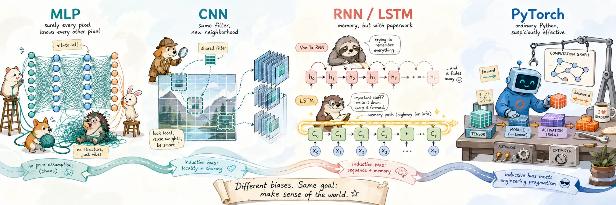
Neural Network Architectures and PyTorch (MLP, CNN, RNN/LSTM)

An architecture is a claim about your data. An MLP claims nothing — every input can interact with every other. A CNN claims that nearby pixels matter to each other and that a pattern is worth detecting wherever it appears. An RNN claims that a sequence is generated by the same dynamics at every step. Machine learning calls these claims inductive biases, and picking an architecture is picking the bias that matches the structure your data actually has: the better the match, the less data you burn teaching the model things you could have built in.

This note covers the three classical families — MLP, CNN, and RNN/LSTM — and then PyTorch, the framework nearly all of it runs on. Two threads run through the whole architecture story and are worth naming up front. The first is weight sharing: a CNN reuses the same small filter at every position in space, an RNN reuses the same transition at every step in time — one idea, two axes. The second is the vanishing gradient: it appears as saturating activations in the MLP, becomes fatal in the RNN, and is finally beaten by an additive path — the same trick, discovered twice, as the LSTM's cell state and as the ResNet's residual connection, and alive today as the residual stream of every transformer.

None of this is taken on faith. The five claims that matter most are each pinned down by a small experiment with real numbers — a widget you can poke at here, and the full training run in the companion lab.

Runnable companion. The Neural Network Architectures lab reproduces every number on this page. Part 1 trains the networks: the depth-versus-width tie, the initialization signal sweep, the learned convolutional filters, the receptive-field arithmetic, the vanishing-gradient measurement with its forget-bias law. Part 2 measures the framework itself: strides, the silent broadcasting bug, the 16-bytes-per-parameter memory arithmetic, the price of backward, the logits overflow, the GPU's lying stopwatch, and what torch.compile actually buys.

---

Foundational Neural Network Architectures

Modern deep learning rests on four families: MLP, CNN, RNN/LSTM, and transformers. Transformers get their own treatment in the LLM track; the three classical families are the subject here — not as history, but because they never left. A transformer block is, in large part, MLP layers wired to attention; convolutions still run most embedded and real-time vision; and all three remain the baselines everything new must beat. More importantly, the mechanisms — weight sharing, gating, additive paths, receptive fields — are the vocabulary in which every modern architecture is written.

MLP — Multi-Layer Perceptron

MLP, or fully-connected network, is the simplest neural network and the base everything else builds on. It is a stack of fully-connected layers, each an affine map $y = Wx + b$ followed by an element-wise nonlinear activation. For a layer with input dimension $d_\text{in}$ and output $d_\text{out}$ the weight matrix is $W \in \mathbb{R}^{d_\text{out} \times d_\text{in}}$ and the bias $b \in \mathbb{R}^{d_\text{out}}$; on a batch of $B$ examples the whole layer is a single matrix multiply, $Y = XW^\top + b$ with $X \in \mathbb{R}^{B \times d_\text{in}}$. "Depth" is just how many of these you stack.

The nonlinearity is not garnish — it is the entire reason a stack is more than one layer. Compose two affine maps with nothing between them and you get $W_2(W_1x + b_1) + b_2 = (W_2 W_1)x + (W_2 b_1 + b_2)$, which is one affine map. Any number of linear layers, however wide, collapses to a single linear model whose decision boundary is a straight line. That is a theorem, but it is more convincing as a measurement — three networks, same ≈907-parameter budget, on a two-spiral task. Hit replay and watch all 6000 epochs: the linear stack's boundary only rotates in place — it cannot bend, no matter how long you train it — while the ReLU nets wrap around the spiral:

The linear stack lands at 55% accuracy — chance level for this data — and no amount of training moves it, exactly as the algebra says: its 907 parameters collapse to one line in the plane. Add ReLU between the same layers and the single-hidden-layer net reaches 0.87 ± 0.06 across seeds (best run 0.96). And here is the honest correction to a popular myth: the five-layer narrow net, same budget, scores 0.87 ± 0.07 — a dead heat. Depth is not automatically better. On a low-dimensional task, width substitutes for depth exactly as the universal approximation theorem promises: one hidden layer of sufficient width can approximate any continuous function. Depth earns its keep on high-dimensional, compositional data — images, language — where each layer can reuse features built by the one below, not on a 2-D spiral. ("Sufficient width," meanwhile, can mean an absurd number of neurons, which is the theorem's own escape hatch — it guarantees existence, not efficiency.)

Activation functions. Historically popular were sigmoid, $\sigma(x) = \tfrac{1}{1+e^{-x}}$ (range $[0,1]$), and tanh (range $[-1,1]$); both are now rare in hidden layers because they saturate — for inputs large in absolute value the derivative is near zero, and a near-zero factor multiplied into the chain rule at every layer shrinks the gradient geometrically. This is the first appearance of the vanishing-gradient thread, and it will return with teeth in the RNN section. The modern default is ReLU, $\max(0, x)$: cheap, and its derivative is exactly $1$ on the positive side, so it passes the gradient through undamped. Its variants — Leaky ReLU (small negative slope, avoids "dead" neurons stuck at zero), GELU (a smooth ReLU, standard in transformers), SwiGLU (a gated variant in modern LLMs) — matter less than the architecture around them; GELU or SwiGLU is a fine default.

Initialization is not a footnote. A forward pass multiplies by a weight matrix per layer, so the scale of initial weights compounds: too large and activations explode with depth, too small and they vanish before the loss ever sees them. The fix is variance bookkeeping — set $\text{Var}(W) = 1/d_\text{in}$ (Xavier/Glorot, for tanh) or $\text{Var}(W) = 2/d_\text{in}$ (He/Kaiming, for ReLU; the factor of two pays for ReLU zeroing half its inputs) so that signal magnitude is preserved layer to layer. How much this matters is easy to state and better to measure — a 40-layer ReLU net on a real MNIST batch, at half the He scale, exactly it, and double it:

The geometry is merciless: each layer multiplies the signal's scale by a near-constant factor, so at half the He scale the activations reach layer 40 at $\sim\!10^{-12}$, at double they blow up to $\sim\!10^{+12}$, and at exactly He they ride flat at std ≈ 1 — and the backward gradient inherits the same three fates. One constant in the init, twelve orders of magnitude at the far end; the difference between a net that trains and one that is dead before the first step. It is one of the quiet reasons deep learning started working at all. But note what initialization buys: a good starting point, nothing more. Past a few dozen layers even well-initialized plain stacks degrade, and fixing that takes an architectural change we will meet in the CNN section.

In practice an MLP is either a baseline (on tabular data it usually loses to gradient boosting, whose tree-shaped bias fits that structure better) or a component inside something larger. A transformer block alternates attention with an MLP — two fully-connected layers around a nonlinearity — and that MLP holds roughly two-thirds of the block's parameters; when you pay for a modern LLM you are mostly buying fully-connected layers. N-BEATS, an MLP stack, held state of the art in time-series forecasting for years; recommenders score with MLP heads; autoencoders are often MLP encoders and decoders. The pattern: an MLP rarely suffices alone on structured data, because claiming nothing about structure means learning all of it from scratch — but it is almost always present.

CNN — Convolutional Neural Network

CNN is the architecture whose claim is local structure plus translation symmetry. The canonical case is images: a cat's ear is a local arrangement of edges, and it is the same arrangement wherever it sits in the frame, so the detector for it should be small and reused everywhere. Worth being precise, because it is a common slip: convolution is translation-equivariant — shift the input and the feature map shifts with it — and it is pooling (or a final global average) that later converts some of that equivariance into invariance, where the answer stops moving at all.

An MLP exploits neither property, and the price is concrete: wiring a 224×224×3 image (150,528 inputs) to a 1000-unit layer costs 150,529,000 parameters — for the first layer. A convolutional layer of 64 filters, each 3×3×3, does its first pass over the same image with 1,792 parameters: a factor of ~84,000, four orders of magnitude, from two ideas — local connectivity (a neuron sees a small patch, not the whole image) and shared weights (the same patch-detector is reused at every position). This is the weight-sharing thread: the parameters no longer scale with image size at all.

Convolution is the operation that implements the claim. A small window — a kernel or filter, typically 3×3, 5×5 or 7×7 — slides across the input; at each position it takes the element-wise product with the patch under it and sums. One kernel, one local feature — an edge at some orientation, a corner, a blob; a layer runs a few dozen in parallel. Nobody designs these features, and you do not have to take that on faith either — here are the eight 7×7 filters a real CNN learned on MNIST, next to the parameter arithmetic above. Reading a filter is simple once you know the code: blue cells are negative weights, warm cells positive, and the filter fires wherever the ink lines up with its warm band — a warm stripe flanked by blue is an edge detector at that orientation. Every feature map here is the actual convolution, running live in your browser with the learned weights:

They emerge as oriented stroke and edge detectors — nobody specified them; gradient descent found them because they are what digits are made of. A handwritten digit contains every orientation at once, which hides the specialization — so probe with the clean strokes: press ╱ and watch most filters go dark while the diagonal specialists light up; switch to │ and the winners change. Then nudge the input with the arrows: the feature map moves with it, pixel for pixel — translation equivariance, the symmetry claim the whole architecture rests on, not as a slogan but as something you just did. Hover the input to see the mechanism itself — the 7×7 window that slides everywhere and produces exactly one map pixel per position. And draw your own digit: the same 49 weights light up on your strokes, because a detector shared across every position has no idea (and no need to know) whose handwriting it is looking at. This particular net reaches 98.5% test accuracy after six epochs — the full training run is in the lab.

Two parameters control the geometry of the output. Stride is how far the kernel jumps per step (stride 2 halves resolution); padding adds a border of zeros so the kernel can sit over edge pixels. For input size $W$, kernel $K$, padding $P$, stride $S$, the output side is $\left\lfloor \frac{W - K + 2P}{S} \right\rfloor + 1$ — the arithmetic every "shape mismatch" bug comes down to. From it follows the quantity that governs what a deep CNN can see: the receptive field, the region of the input that influences a single deep neuron. How fast it grows with depth is entirely a function of stride and pooling, and the difference is dramatic:

The numbers are the argument. A plain stack of 3×3 convolutions grows its receptive field by +2 per layer — after 12 layers a neuron sees a 25-pixel patch, and covering a 224-pixel image would take 112 layers. Interleave a 2×2 pooling after every pair of convolutions and by the same 12 operations the receptive field is 76 pixels and each further layer adds 32 more, because every downsampling doubles the step between neighboring neurons. That is the real job of stride and pooling: not "reducing computation" (a side benefit) but buying receptive field cheaply. The same widget carries VGG's famous observation: two stacked 3×3 kernels see the same 5×5 patch as one 5×5 kernel at 18 parameters versus 25 — with two nonlinearities instead of one; three 3×3 layers match a 7×7 at 27 versus 49. Stacked small kernels are strictly the better deal, which is why nearly every modern CNN is built from 3×3s.

Pooling itself is simple — max pooling takes the maximum over a window (usually 2×2), average pooling the mean — and it is where translation invariance enters: nudge the cat one pixel and the max over the window does not flinch. Modern architectures often swap pooling for a stride-2 convolution: same downsampling, learnable weights.

The history of CNNs is best read not as a parade of names but as one question asked repeatedly: how deep can you train? LeNet (1998) proved the concept at 7 layers. AlexNet (2012) got to 8, won ImageNet by a margin that started the deep learning era, and made GPUs standard equipment. VGG (2014) reached 19 by committing fully to stacked 3×3 kernels — the arithmetic above. And then progress hit a wall that had nothing to do with overfitting: past roughly 20 layers, adding depth made even the training error worse. A 56-layer plain net trained worse than a 20-layer one — an optimization failure, the vanishing-gradient thread again, now killing networks in open daylight despite good initialization and ReLU. ResNet (2015) broke the wall with one structural move: let each block compute a correction to its input rather than a replacement, $y = x + F(x)$. The identity path is additive — no weight matrix on it, nothing to attenuate — so the gradient flows backward through $+\,x$ undamped no matter how many blocks it crosses, and 152-layer networks suddenly trained without drama. Hold that thought: an additive path that gradients can ride without being multiplied by weights — the RNN section is about to show the same idea invented eighteen years earlier along the time axis, and every transformer alive carries it today as the residual stream. EfficientNet (2019) then made depth-width-resolution scaling systematic, but the load-bearing discovery was ResNet's.

In recent years Vision Transformers (ViT) have displaced CNNs at the top of leaderboards, and the reason is the inductive-bias trade running this whole note: a ViT discards the locality-and-translation prior and lets attention learn pixel relationships from scratch — which loses when data is modest (the prior was doing real work) and wins when data is abundant (the prior becomes a straitjacket; attention finds relationships convolution cannot express). That is why CNNs remain the practical choice for most real deployments — faster to train, happier on small data and small hardware, still the workhorse of segmentation, detection, OCR, and nearly all embedded vision — while ViTs rule the large-data regime.

And CNNs are not only for images. The claim "local patterns, position-independent" holds for any data on a grid: 1D convolutions over audio waveforms and time series (the Temporal Convolutional Network, covered in the time-series track) and — before transformers — over text; 3D convolutions over video and volumetric medical scans. Same bias, different number of axes.

RNN, LSTM, GRU — Recurrent Networks

RNN (Recurrent Neural Network) is the architecture whose claim is sequential structure: the data arrives as a sequence, and the same dynamics generate every step. It processes elements one at a time, carrying an internal state $h_t$ between steps: at step $t$ it combines the current input $x_t$ with the previous state $h_{t-1}$ and updates, the simplest form being $h_t = \tanh(W_h h_{t-1} + W_x x_t + b)$. The same $W_h$ and $W_x$ are reused at every step — weight sharing again, along time instead of space — which is what lets one small network handle sequences of any length.

That same reuse is the source of the architecture's defining failure. Training uses backpropagation through time (BPTT): unroll the network across the sequence, run the gradient back through every step. Chaining the recurrence, the gradient of a late state with respect to an early one is a product with one factor per step:

$\dfrac{\partial h_t}{\partial h_k} = \prod_{i=k+1}^{t} \operatorname{diag}\!\big(\tanh'\big)\, W_h^{\top}$

A product of $t-k$ near-identical factors is an exponential in $t-k$: if the largest singular value of $W_h$ (times the tanh derivative, which is at most 1) sits below one, the product collapses geometrically; above one, it explodes. There is no stable middle — and unlike the MLP case, initialization cannot save you, because the same matrix is applied at every step. Explosions have a crude but effective fix, gradient clipping (rescale the gradient when its norm exceeds a threshold); vanishing has no such patch, and it is worth seeing how brutally fast it bites. Measured on real cells — 32 hidden units, 16 seeds, a 60-step sequence, tracking how much gradient from the final loss survives the trip back to each earlier step. The slider is the experiment: it sets the LSTM's forget-gate bias, and you open the gradient highway yourself:

The vanilla RNN's gradient is down to $3\times10^{-4}$ of its strength just ten steps back, $\sim\!10^{-10}$ at thirty, $\sim\!10^{-19}$ at sixty — for learning purposes, anything past about ten steps might as well not exist. This is not a tuning problem; it is the geometry of multiplying sixty matrices together.

LSTM (Long Short-Term Memory) (Hochreiter & Schmidhuber, 1997) beats it with a gating mechanism and a second state. Alongside $h_t$ it carries a cell state $c_t$ — the long-term memory. Three gates, each a small sigmoid layer over $[h_{t-1}, x_t]$ producing values in $[0,1]$, control the traffic:

$f_t = \sigma(W_f[h_{t-1}, x_t] + b_f), \quad i_t = \sigma(W_i[h_{t-1}, x_t] + b_i), \quad o_t = \sigma(W_o[h_{t-1}, x_t] + b_o)$ $\tilde{c}_t = \tanh(W_c[h_{t-1}, x_t] + b_c), \qquad c_t = f_t \odot c_{t-1} + i_t \odot \tilde{c}_t, \qquad h_t = o_t \odot \tanh(c_t)$

The forget gate scales how much old memory survives, the input gate how much new content is written, the output gate what leaks out as $h_t$. The one line that matters is the cell update, $c_t = f_t \odot c_{t-1} + i_t \odot \tilde{c}_t$: it is additive — an element-wise gate-and-add with no weight matrix in the path. Recognize it? It is ResNet's $y = x + F(x)$, invented for time instead of depth. The cell state's step-to-step derivative is simply $\partial c_t / \partial c_{t-1} = f_t$ — a multiply by the forget gate, nothing else — so the gradient along the cell path is a product of forget gates rather than of $W_h$, and when the gates sit near 1 it rides back across the whole sequence almost undamped. The classic name for this is the constant error carousel.

But the measurement above holds an honest subtlety the textbook story skips. Set the slider to 0 — effectively the default initialization — and the LSTM's curve also decays, $\sim\!10^{-7}$ by thirty steps. Why? With zero bias the forget gates start at $f_t \approx \sigma(0) = 0.5$, and a product of 0.5s is still an exponential decay ($0.5^{10} \approx 10^{-3}$ — almost exactly where the measured curve sits at ten steps). Gating enables long memory; it does not grant it at birth — the network must learn to hold its gates open, and early in training the gradient it needs to learn that with is itself decaying. Hence the classic trick: bias the forget gate open at initialization. Drag the slider and watch the theory track the measurement decade by decade — each unit of bias lifts the floor by orders of magnitude, because the gradient goes like $\sigma(b_f)^k$: at $b_f = 1$ the 60-step reach is $\sim\!10^{-6}$, at $b_f = 3$ ($f_t \approx 0.95$) it holds at 0.2–0.26 across all sixty steps, and at $b_f = 4$ it barely decays at all. One added constant, six orders of magnitude more gradient at step 30. Theory predicting measurement this cleanly is rare enough to savor.

GRU (Gated Recurrent Unit) (Cho, 2014) is the leaner cousin: two gates instead of three, one state instead of two, comparable quality on most tasks with fewer parameters. The LSTM-vs-GRU choice is secondary; either is reasonable.

Transformers displaced RNNs from most of NLP, and the displacement has a clean mechanistic reading. First, path length: information connecting step 5 to step 500 in an RNN must survive 495 multiplicative updates, while self-attention connects any two positions in one hop — the gradient path is $O(1)$ instead of $O(t)$, dissolving the vanishing problem instead of managing it. Second, parallelism: the recurrence $h_t = f(h_{t-1}, \ldots)$ is inherently sequential — step $t$ cannot begin before $t-1$ finishes — while a transformer processes all positions of a sequence at once, which is the shape of computation GPUs are built for. But where sequences are very long, compute is tight, data is scarce, or inference is streaming — speech, embedded systems, industrial time series — LSTMs remain competitive and regularly beat transformers and foundation models on their home turf.

A detailed treatment of the LSTM applied to time series — every component of the cell, initialization, hybrids with TCN, attention, and N-BEATS heads — lives in the time-series track. The shape to carry from here: RNN is the idea, LSTM is the idea made trainable by an additive path, GRU is the economy version.

Which Architecture Where

The bias-matching rule, made concrete. Tabular data — gradient boosting first; an MLP earns its place at large scale or when fusing several modalities in one model. Images — CNN by default; ViT when data and compute are abundant. Text — transformers, with TF-IDF + a classical model as the honest baseline. Time series — for short series with little data, classical models (ARIMA) or gradient boosting; for rich panels, foundation models (Chronos) or hybrid DL with LSTM/TCN/attention. Audio — CNN over spectrograms; RNN or transformers over raw samples. Graphs — Graph Neural Networks. The boundaries move every year — transformers keep invading (vision, time series, audio) because at sufficient scale learned structure beats built-in structure — but the classical architectures keep winning specific niches for exactly the mirror-image reason.

---

PyTorch: Three Ideas

Strip away the branding and a deep learning framework is three ideas stacked on each other: a tensor library (N-dimensional arrays that run the same code on CPU or GPU), an autograd engine (a tape that records the forward pass and replays it backward for gradients), and a module system (parameters as managed state, plus optimizers to update them). Everything else — data loaders, distributed training, compilers — is service around that core. PyTorch's particular win, and the reason nearly every paper of the last several years ships PyTorch code, is that it made all three feel like ordinary Python.

The design bet is called define-by-run: the computation graph is not declared ahead of time, it is recorded while your code executes. Older frameworks (TensorFlow 1.x) made you describe the graph as a static object, compile it, then push data through — efficient, but you could not set a breakpoint inside a forward pass or use a plain Python if on a tensor's value. In PyTorch the graph is rebuilt on every forward pass, so Python control flow — if, for, variable-length loops — just works, per-sample architecture changes are ordinary code, and debugging is print statements and breakpoints. The industry conceded the point: TensorFlow 2 made eager execution the default, and the modern JAX takes a third path (pure functions, compiled). The trade-off define-by-run gives up — whole-graph optimization — comes back at the end of this note via torch.compile.

Tensor — an array with a device and a memory layout

The central object is the Tensor, an N-dimensional array with NumPy's API plus two additions that matter:

x = torch.tensor([1.0, 2.0, 3.0], device='cuda', requires_grad=True)

device places the data — CPU or GPU — and every operation runs where the data lives. requires_grad=True enrolls the tensor with autograd: from now on, operations on it are recorded.

The mental model worth installing early: a tensor is a data pointer plus shape plus strides. The strides say how many elements to skip in flat memory to advance one step along each axis — and a surprising amount of the API is stride arithmetic on the same memory. transpose, permute, slicing, expand copy nothing: they return a view with rearranged strides. That is why they are free, and also why view() sometimes refuses to work after a transpose — the memory is no longer laid out in the order the new shape implies, and you must call .contiguous() (a real copy) or use reshape() (which copies only when needed). Interop with NumPy is the same story: torch.from_numpy(arr) and tensor.numpy() share memory on CPU, zero-copy.

The other thing to install early is respect for broadcasting. The rule is compact — align shapes from the right; dimensions match if equal or if one of them is 1, which stretches to fit — and it makes most code pleasantly free of explicit loops. It is also the top source of silent bugs in the wild. Subtract a (B,) tensor from a (B, 1) tensor and nothing errors: broadcasting happily produces a (B, B) matrix, your loss averages over it, the number even goes down — and the model is garbage. Nothing crashes; the shapes were merely plausible. The discipline that saves hours: know the intended shape of every tensor in the forward pass, and assert it when in doubt.

Autograd — one backward pass, all the gradients

Autograd is why you can train any model you can write, without deriving a single gradient by hand:

y = x ** 2
loss = y.sum()
loss.backward()
# x.grad now contains d(loss)/dx

Every operation on a tracked tensor appends a node to the graph recording how to transform a gradient flowing out of the op into gradients flowing in — a vector–Jacobian product. Calling .backward() on the scalar loss walks the recorded graph in reverse, multiplying local derivatives by the chain rule, and deposits results in the .grad of every leaf tensor.

Why reverse order? Because training has one scalar loss and millions of parameters. Reverse-mode differentiation propagates from the single output backward and yields all parameter gradients in one sweep, at a cost of roughly 2× the forward pass — independent of parameter count. Forward-mode would need one pass per parameter: a million passes. Reverse-mode is not a convenience; it is the asymmetry that makes gradient descent on huge models affordable at all, and "one scalar out" is why .backward() wants a scalar.

The sweep has a price, and it is paid in memory: to compute those vector–Jacobian products, the backward pass needs the forward pass's intermediate activations, so autograd keeps them alive from forward until backward. That single fact organizes all practical GPU-memory arithmetic. Training a model in fp32 costs, per parameter: 4 bytes of weight, 4 of gradient, and 8 of optimizer state (Adam's two moments — below) — ~16 bytes per parameter before a single activation, roughly four times the model's own size — plus activations proportional to batch size × depth, which for large batches dominate everything. This is why torch.no_grad() at inference is not a micro-optimization (no tape → no stored activations → a fraction of the memory), why the standard OOM fix is a smaller batch, and why gradient checkpointing exists: drop activations during forward, recompute them during backward — memory traded for ~30% more compute.

nn.Module — parameters as managed state

class MyNet(nn.Module):
    def __init__(self):
        super().__init__()
        self.fc = nn.Linear(10, 1)
    def forward(self, x):
        return self.fc(x)

A model is state (weights) plus a function (forward). nn.Module manages the state so you only write the function. The mechanism is attribute registration: assign an nn.Parameter or a submodule to self.anything and the module records it, recursively — so model.parameters() yields every weight in the tree (that iterator is exactly what you hand the optimizer), model.to(device) moves them all, and state_dict() serializes them into a dictionary of named tensors for saving and loading. Your only obligation is forward(); the backward comes from autograd, always in sync with the code you actually wrote — there is no separate "graph definition" to drift out of date.

CUDA — the same code, on the GPU

Moving computation to the GPU is one idiom:

device = 'cuda' if torch.cuda.is_available() else 'cpu'
model = model.to(device)
x = x.to(device)

Model and data must live on the same device — mixing them is an immediate error, one of the friendlier ones — and the is_available() check makes the same script run on a CPU laptop and a GPU server unchanged. The speedup on neural workloads is one to two orders of magnitude, and it comes from a real match: the padded-out matrix multiplies that dominate a forward pass are exactly the massively parallel arithmetic GPUs are built to saturate — the same match that made AlexNet possible.

Two things about the execution model save real debugging time. First, CUDA is asynchronous: Python queues kernels and returns immediately while the GPU works through them, so wrapping a forward pass in time.time() measures how fast you enqueue, not how fast the GPU computes — call torch.cuda.synchronize() before reading the clock. Second, the scarce resource is often not GPU arithmetic but the PCIe transfer feeding it: moving data from host to device is slow relative to compute, which is why the discipline is to move data once and keep it there, and why the DataLoader below has a pin_memory flag. For multi-GPU, DistributedDataParallel (DDP) is the modern standard; the older DataParallel survives only for quick experiments.

Optimizers — what Adam actually does

torch.optim holds the update rules. SGD is the reference point: parameters step against the gradient, usually with momentum (an exponential moving average of gradients that smooths the descent direction). Adam's pitch is a per-parameter step size: it keeps a running mean of each gradient (first moment) and a running mean of its square (second moment), and divides the step by the square root of the latter — so a parameter with consistently large gradients takes careful small steps and a rarely-updated one takes bold ones. Those two moments are the 8 bytes per parameter from the memory arithmetic above — the price of adaptivity, paid in VRAM.

AdamW fixes a subtle bug in how Adam does weight decay. Classic L2 regularization adds the penalty to the gradient, which in Adam then gets divided by that same adaptive denominator — so precisely the weights with large gradient history, often the ones most in need of shrinking, are barely decayed at all. AdamW decouples the decay, applying it directly to the weight, outside the adaptive machinery. The difference looks minor and reliably is not; AdamW is the default for training transformers, and a sensible default overall.

Whatever the optimizer, the learning rate is the one hyperparameter that always matters — too high diverges, too low crawls into a poor solution — and in serious training it is scheduled rather than fixed (warmup then cosine decay is the standard recipe for transformers).

Loss functions — and one numerical trap

Losses live in torch.nn: MSELoss for regression, L1Loss when outliers must not dominate, SmoothL1Loss (Huber) as the compromise, CrossEntropyLoss for multi-class classification, BCEWithLogitsLoss for binary. A custom loss is just a Python function whose output is a differentiable tensor — autograd handles the rest.

One design decision deserves its mechanism spelled out: CrossEntropyLoss takes raw logits, not softmax outputs, because it fuses softmax and negative log-likelihood internally — and the fusion is numerics, not tidiness. Softmax exponentiates, and in float32 $e^x$ overflows to infinity around $x \approx 89$ — logits a confident model produces without effort. The fused version uses the log-sum-exp identity, subtracting the max logit before exponentiating (which changes nothing mathematically and everything numerically), and stays stable at any confidence. Apply your own softmax first and you both break the stabilization and feed the loss a double-softmax. BCEWithLogitsLoss versus BCELoss is the same story — always the logits version.

DataLoader — keeping the GPU fed

DataLoader turns a dataset into an iterator of batches:

from torch.utils.data import DataLoader

loader = DataLoader(
    dataset,
    batch_size=32,
    shuffle=True,
    num_workers=4,
    pin_memory=True,
)

Batching and per-epoch shuffling are the visible features; the load-bearing ones are the other two. num_workers runs data loading in parallel worker processes so the next batch is ready before the GPU finishes the current one, and pin_memory stages batches in page-locked host memory from which host-to-device copies run fast and asynchronously — the PCIe story from the CUDA section, addressed at the source. The failure mode this machinery exists for is mundane and expensive: an idle accelerator waiting on I/O. When training is slow, profile the input pipeline before blaming the model — a starved GPU looks exactly like a slow one.

The training loop, end to end

Every abstraction above exists to serve one small ritual. Here it is whole — the CNN from the architecture section, trained on real images; this exact code, executed, is what produced the learned filters in the widget above:

import torch, torch.nn as nn, torch.nn.functional as F

class CNN(nn.Module):                     # the architecture, in code
    def __init__(self):
        super().__init__()
        self.c1 = nn.Conv2d(1, 8, 7, padding=3)     # 8 learned 7×7 filters
        self.c2 = nn.Conv2d(8, 16, 3, padding=1)
        self.fc = nn.Linear(16 * 7 * 7, 10)
    def forward(self, x):                 # only the forward pass — autograd does the rest
        x = F.max_pool2d(F.relu(self.c1(x)), 2)      # conv → ReLU → pool
        x = F.max_pool2d(F.relu(self.c2(x)), 2)
        return self.fc(x.flatten(1))                 # logits, not softmax

device = "cuda" if torch.cuda.is_available() else "cpu"
model = CNN().to(device)
opt = torch.optim.AdamW(model.parameters(), lr=1e-3)

for epoch in range(6):
    model.train()                         # enable dropout / batchnorm-train behaviour
    for xb, yb in train_loader:
        xb, yb = xb.to(device), yb.to(device)        # data must sit on the model's device
        opt.zero_grad()                   # clear last step's gradients (they accumulate)
        loss = F.cross_entropy(model(xb), yb)        # forward + loss, on raw logits
        loss.backward()                   # autograd fills every .grad
        opt.step()                        # nudge each parameter down its gradient

    model.eval()                          # switch to inference behaviour
    correct = 0
    with torch.no_grad():                 # no tape, no stored activations — fast and lean
        for xb, yb in test_loader:
            correct += (model(xb.to(device)).argmax(1).cpu() == yb).sum().item()
    print(epoch, correct / len(test_loader.dataset))

Four lines carry the learning — zero_grad, forward-and-loss, backward, step — and in the lab this loop reaches 98.6% test accuracy in under twenty seconds on a plain CPU. Three details trip up everyone at least once. Gradients accumulate across backward() calls unless zeroed — a feature (it lets you simulate large batches by accumulating over several small ones) and a bug magnet. model.train() versus model.eval() flips dropout and batch-norm into the right regime; forgetting it silently corrupts evaluation. And torch.no_grad() at inference is the memory-arithmetic section cashed in: same forward, no tape. (One more, for recurrent nets specifically: clip_grad_norm_ between backward and step — the exploding-gradient patch from the RNN section, one line here.) In practice this loop appears in three sizes — inference with a pretrained model (forward pass only), fine-tuning (freeze most of it, retrain the head), and training from scratch — and it is the same loop each time, with more of it under your control.

torch.compile — buying back the compiler

Define-by-run traded whole-graph optimization for flexibility. PyTorch 2.0 (2023) bought it back:

model = torch.compile(model)

To see why this helps, note what eager mode actually costs: one kernel launch per operation, and — the dominant term — a round trip to GPU memory for every intermediate result, because most tensor ops (activations, normalizations, elementwise arithmetic) are memory-bandwidth-bound, not compute-bound. The GPU spends its time ferrying tensors to and from HBM, not multiplying. torch.compile captures the graph by tracing Python bytecode (TorchDynamo) and generates fused kernels (TorchInductor) — chains like conv → bias → ReLU become one kernel, intermediates never leave fast on-chip memory, and typical models get 1.3–2× essentially for free. Where tracing meets something it cannot capture (arbitrary Python side effects, data-dependent control flow), it inserts a graph break and falls back to eager for that stretch — correctness is preserved, speedup shrinks. This closed the last real performance argument for static-graph frameworks.

---

The Landscape, Briefly

TensorFlow remains the second mainstream framework, strongest where its serving and mobile ecosystem (TF Serving, TF Lite) is entrenched, but it has effectively ceded research. The interesting pole is JAX: NumPy semantics plus composable function transforms — grad, jit, vmap — over pure functions, aggressively compiled via XLA; it is what you reach for when compilation and TPUs dominate the problem, at the cost of a stricter functional style (with Flax and Equinox as its neural libraries, and Keras floating above several backends as a high-level API). For most work the answer is PyTorch, and not by inertia: the ideas this note is built from — tensors with autograd, modules as state, a tape you can debug through — are simply its native vocabulary.

That is the note. Three architectures, each an inductive bias you can state in one sentence; two threads — weight sharing and the additive path — that reappear from CNNs to LSTMs to every transformer running today; and a framework that reduces to a tensor, a tape, and a module. Every number along the way was measured, and the companion lab will re-measure them for you: change a width, close a forget gate, break the spiral — the fastest way to make any of this stick is to make one of the plots come out differently and understand why.