Isotonic Regression on GPU

A Tesla T4 has 2,560 cores. Ask it to fit ten million numbers with a curve that is only allowed to go up, using the exact solver that differentiable-sorting libraries ship, and it needs five and a half seconds. An A100, a far bigger GPU, needs six and a half. One core of an ordinary CPU needs a sixth of a second.

More hardware, a slower answer. Nothing is broken: the solver is a loop of about ten lines that walks the numbers from left to right, and a walk is the one thing a GPU cannot share out among its thousands of threads.

My library torchisotonic and its paper, Merge Hulls Without Copying Vertices: GPU Isotonic Regression, are an answer to that puzzle. On the same T4 the same ten million numbers now take about two milliseconds, and not because anyone made the walk faster.

Code: github.com/LenaBarretta/torchisotonic · Paper: arXiv 2610.24038 · Install: pip install torchisotonic

The walk was never the point. The answer turns out to have been a picture all along, a string pulled tight under a row of nails, and a picture, unlike a walk, can be drawn in pieces. Then comes the lesson every note in this track keeps arriving at from a different side: once the pieces are drawn, gluing them together costs almost no arithmetic and an enormous amount of copying, and the fix is not to copy faster but to stop moving things that never change.

Most of these ingredients are classical: the string, the pieces, the gluing. My part is the last step, how to store glued pieces so that gluing them on a GPU moves almost nothing, together with a proof that the storage is correct, the CUDA operator and its measurements on four GPUs.

A model that believes only in order

Most models assume a lot about the world: a straight line, a curve of a chosen shape, a network of a chosen size. Isotonic regression assumes one thing only — that more of the input should never mean less of the output. A higher score, never a lower probability. A better match, never a worse rank. Everything else it takes from the data.

That makes it the tool people reach for when a model's numbers are right in order but wrong in scale. Click models in advertising are the classic case. They are usually trained on data from which nine non-clicks out of ten were thrown away, because there are so many of them, so the model comes out optimistic: an ad that people really click 0.4% of the time is predicted at about 4%. That is not a bug in the model; it is arithmetic. Before anyone bids money on those predictions, a curve fitted on a day of real traffic maps what the model said to what actually happened, often hundreds of curves at once, one per country or campaign. The one rule the curve may not break is the order.

The same humble assumption sits inside training. Differentiable sorting and ranking, the tools that let a model learn directly from getting an order right, solve an isotonic regression in every forward pass and reuse its blocks in the backward one. There a slow solver is not an inconvenience at the end of a pipeline. It is a tax on every step.

A curve that is only allowed to go up

It helps to see what the numbers are. Sort a day's impressions by the model's score; the score decides the order and nothing else. The values to fit are what happened, in that order: 1 for a click, 0 for none, something like 0, 0, 0, 1, 0, 0, 1, 0, 1, 1. A curve that may only go up, fitted to those zeros and ones, turns them into a click rate that rises with the score: 0 for the three lowest scores, a third for the next three, a half for the two after, 1 for the top two. That fitted value is the calibrated probability for each score.

Strip the advertising away and the problem is this. You have a sequence of numbers $y_1, \dots, y_n$. Find the sequence $x_1 \le x_2 \le \dots \le x_n$ closest to it, in the sense of the sum of squared differences. Where the data already go up, the answer is the data. Wherever they go down, the answer has to flatten out.

The algorithm that solves it is called pool adjacent violators, PAVA for short. Walk left to right. Every value starts as a block of its own. Whenever a block's average is lower than the average of the block before it, the two "violate" the order: merge them into one block whose value is their combined average. Then look back again, because the merged block may now violate its left neighbour.

def isotonic(y):
    blocks = []                         # each block: [sum, count]
    for v in y:
        blocks.append([v, 1])
        # while the last block's mean is below the one before it, pool the two
        while len(blocks) > 1 and blocks[-1][0] / blocks[-1][1] < blocks[-2][0] / blocks[-2][1]:
            s, c = blocks.pop()
            blocks[-1][0] += s
            blocks[-1][1] += c
    return [s / c for s, c in blocks for _ in range(c)]

Try it on [1, 3, 2, 4]. The 3 and the 2 violate the order, so they become one block of 2.5, and the answer is [1, 2.5, 2.5, 4]. Now try [5, 1, 2, 3]: 5 and 1 pool into 3, then the 2 arrives, is below 3, and pulls the block further down, to $(5+1+2)/3 \approx 2.67$. The answer is [2.67, 2.67, 2.67, 3]. The value in third place changed the answer in first place.

Every value enters the stack once and leaves it at most once, so the whole thing is linear in $n$. On a CPU it is about as fast as an algorithm can be.

Why a bigger GPU does not help

Look at that second example again: the first element's final value was not known until the third had been read. In general a block is not settled until everything to its left is settled, and possibly not even then, because one small value far to the right can pull a whole run of blocks down. Each step depends on the one before. That is a chain, and a chain runs on one thread.

The natural GPU design accepts this and finds its parallelism elsewhere: one thread per row. With a million short rows that is a million threads, and the GPU is busy. With one long row it is the worst design there is. As How GPUs Actually Run Machine Learning works out, a GPU is fast because it keeps tens of thousands of threads in flight and switches between them while each one waits for memory. A single thread has nothing to switch to. It waits for every access in full, on a core clocked lower than a CPU core and built for throughput rather than for speed on its own.

one row of 10⁷ values	time
one thread per row, Tesla T4	5.5 s
one thread per row, A100	6.4 s
one thread per row, H100	4.7 s
pool adjacent violators, one CPU core	0.17 s

One row of 10⁷ float32 values, a rising trend plus noise, already in GPU memory. The GPU lines are torchsort's solver, the one differentiable-sorting libraries use; the CPU line is SciPy's compiled pool adjacent violators, not the Python above.

That is also why the size of the GPU stops mattering: one thread uses almost none of any of them.

The third view is where this note is heading: cut the row into chunks so that the whole GPU has something to do, then glue the pieces back together in a tree whose upper levels need only a sliver of it. To get there, the problem has to stop being a chain, and no amount of speeding up the chain will do that.

Nails and a string

Instead of the values, write down their running totals, and treat each total as a point: the first point at height 0, the next at the first value, the next at the sum of the first two, and so on. For [1, 3, 2, 4] the totals are 0, 1, 4, 6, 10.

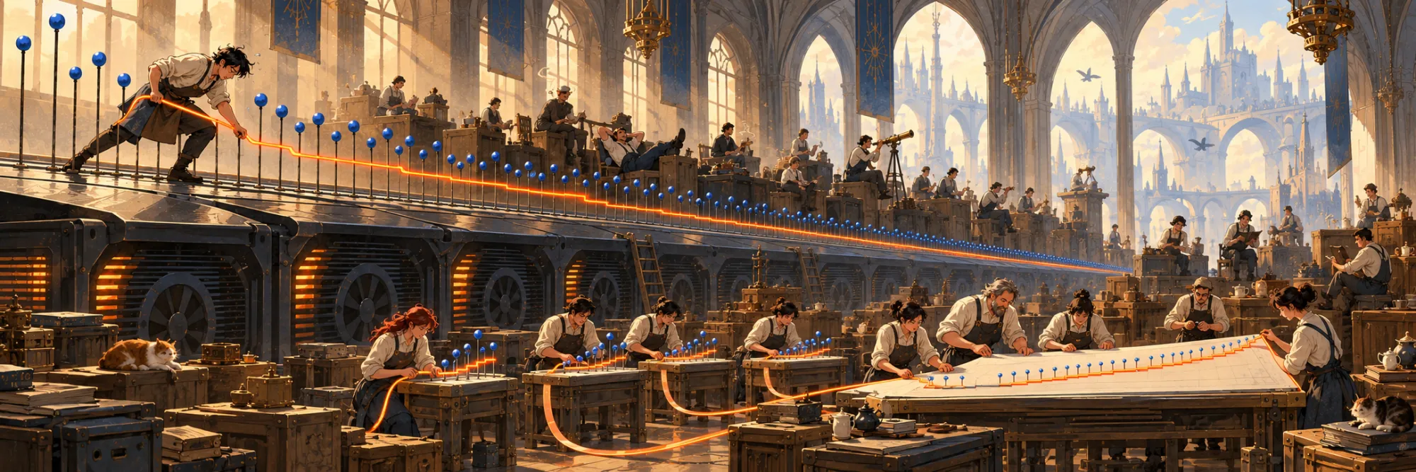
Now picture those points as nails in a board, and pull a string tight underneath them, from the first nail to the last. The string touches some nails and passes under others. Read off the slopes of its pieces, and you have the isotonic fit.

Why that works fits in three sentences. The slope between two nails is the average of the values between them, which is exactly what pool adjacent violators assigns to a block. A drop in the data bends the running total the wrong way and lifts a nail above the straight line between its neighbours; a string pulled tight from below does not climb over that nail but passes beneath it in a straight line, and following the straight line instead of the nails is exactly averaging the values it spans. And a string pulled tight from below can only bend upwards, so its slopes never decrease — which is the rule the curve had to obey.

Run the build from left to right in the widget and the two are not just equal at the end, they are equal at every step. Each time pool adjacent violators pools two blocks, the string lets go of a nail. The walk was building this string all along, one nail at a time.

The shape the string makes has a name, the lower convex hull of the points, and the equivalence is a classical result in statistics. It changes the question. Not "walk the data and pool violators" but "find the bottom edge of a cloud of points" — and a hull, unlike a walk, can be built in pieces.

Glue the pieces

Split the points into chunks. Each chunk's hull can be built on its own, knowing nothing about the others. Then glue neighbouring hulls together in pairs: eight become four, four become two, two become one. Every gluing at the same level is independent of all the others, so they run at the same time, and a row of $m$ chunks needs only about $\log_2 m$ levels.

Gluing two hulls, one entirely to the left of the other, means finding the bridge: the one segment that touches both hulls and has every point above it. The merged hull is the left hull up to the bridge, the bridge itself, and the right hull from there on. Everything between the bridge's two ends falls off.

Two things are worth noticing in that picture. The first is that the merged hull contains no new points: it is a stretch of the left hull, a stretch of the right hull, and one new segment between two nails that were already there. That observation is the one the rest of this note turns on.

The second is less comfortable. Usually the bridge turns up within a handful of steps of where the two hulls meet. But choose a cliff at the end in the widget: one value far below drags the bridge across the whole picture, and the walk visits nail after nail, one after another. The sequential walk this note set out to escape is back, inside the merge. Inside a chunk that is tolerable, since a walk there can never be longer than the chunk's 1,024 points. Between chunks a hull can have millions of vertices, so there torchisotonic does not let a merge walk freely. A merge done by a single thread walks at most 64 steps and, if the bridge has not turned up by then, finds it by binary search over the candidates, a search that grows only with the logarithm of the hull. The few merges at the top of the tree, done by a whole warp, search from the start.

A whole stack in one register

The pieces map onto the GPU at three sizes.

The smallest is a lane, one thread of a warp, which takes 32 consecutive points and builds their hull with the same walk as before. The walk is still sequential, but over 32 points it is short, and the 32 lanes of a warp run it side by side, each on its own 32 points. The stack it needs fits in a single register: one bit per point, set while that point is on the stack.

A push sets a bit and a pop clears one. The top of the stack and the entry under it also stay in registers, so testing the next point needs no lookup at all; when the top comes off, the new entry under it is the highest set bit below the old one, which a single count-leading-zeros instruction finds. Every pass through the loop either pops or pushes and makes both loads it might need, so the loop has no branch that depends on the numbers, apart from a rare slow path in float32 that rechecks a turn too close to call: the 32 lanes of a warp stay in step, and the stack never touches memory.

Above the lanes, the lanes of a warp glue their hulls in shared memory into the hull of a chunk of 1,024 points — by clearing bits, not by copying: a vertex that falls under a bridge inside a chunk simply has its bit set to zero. Above the chunks, the chunks of a long row glue theirs up a tree, in global memory. Everything below that last level is fast and local. The last level is where the cost hides.

The trap: copying what survives

The obvious way to store a hull is an array of its vertices. Then a merge produces a new array: the surviving vertices of the left hull, then the surviving vertices of the right one, written out one after the other. That is how a textbook would write it, and it is correct.

Now think about how many vertices survive. On noisy data the hull is sparse: most points sit above the string, each chunk's hull has a few vertices, and after a couple of merges there is almost nothing left to copy. But if the data already go up, the running totals bend upwards everywhere and every point is a vertex. A merge then drops almost nothing, and the next level copies almost the whole row again, and the next.

Count it for one increasing row of ten million values. With chunks of 1,024 points there are 9,766 chunks and 14 levels of merging. A copied vertex takes 16 bytes, its height, its position and the chunk it came from, so a level that writes out every merged hull writes 160 MB, and the merge tree writes 2.2 GB — and reads as much — to produce an answer of 40 MB. The arithmetic of a merge is a few comparisons near the bridge. The copy is nearly the whole cost, which is what Matrix Multiplication found for a completely different operation: on a GPU, you pay for bytes.

Copying faster helps, up to a point. In the textbook merge, the thread or warp that found the bridge moves the right hull's survivors down behind the left one's. That writes only half as much, 1.0 GB, and still takes 171 ms for the merge stage on a T4: at the top of the tree a single warp copies millions of vertices on its own, the narrow top of the pipeline in the widget further up. A separate kernel that rewrites every merged hull with the whole GPU and coalesced accesses, at half to two thirds of the card's peak bandwidth, writes the full 2.2 GB and brings the stage to 25 ms. Both are still copying vertices that never changed.

Keep the vertices where they are

Go back to the bridge. A merge never changes a vertex. A vertex stays on the hull or falls off it; it never moves, and nothing new appears except the bridge, which joins two vertices that already exist. So there is no reason to move them.

Each chunk writes its hull's vertices once, into a slot of its own, and they stay there to the end. A merged hull is then not an array of points but a short list of segments, each one saying "chunk 3, vertices 2 to 6", then "chunk 4, vertices 0 to 7". A merge finds the bridge, trims the two segments the bridge touches, and appends the right list to the left one. A few small numbers change. Not one vertex moves.

What makes this safe is a fact that is not obvious at first: a merged hull never needs more than one segment per chunk. You might worry that a chunk's surviving vertices end up scattered in several pieces. They cannot. The merged hull runs left to right, and a chunk's points occupy one stretch of it. Two neighbouring vertices of the merged hull inside that stretch are joined by an edge that lies under every point, the chunk's own points included, so they are neighbours on the chunk's own hull as well. That fixes the space for the lists in advance: one descriptor slot per chunk, 24 bytes each.

On that increasing row the merges now move 1.5 MB of descriptors instead of gigabytes of vertices, and even most descriptors stay put, since a merge moves only the right list. The merge stage on a T4 takes 0.19 ms instead of 25. The whole operator, with its other stages, is nine times faster on the T4 and about four times faster on an A100 or H100, whose memory is several times quicker and makes copying cheaper. Cheaper, not free.

If this looks familiar, it should. PagedAttention does the same with a language model's cache: instead of copying a conversation's keys and values into one contiguous buffer as it grows, it keeps them in fixed blocks and a table that points at them. Operating systems did it decades earlier with page tables, and the classic dynamic hull structures, balanced trees that relink their nodes at a bridge, never copy vertices either; segment lists are the flat form of that idea, one descriptor slot per chunk, which is the form a GPU wants. A table of contents instead of retyping the book: whenever the thing you are building is made of pieces that never change, store where the pieces are, not the pieces.

Where the gain is smaller

On noisy data, the trap is not much of a trap. Few vertices survive the first merges, so copying them was already cheap, and there is little left for segment lists to save. On a noisy row of ten million on the T4, the merge stage takes about half a millisecond either way. The whole operator is still about 10% faster, but that comes from the rest of the pipeline, not the merges. Only at a hundred million noisy values do the segment lists pull ahead again, by one and a half to two times.

That is worth saying out loud. Segment lists buy most where many vertices survive, in data that is already nearly in order, and which case a workload falls into depends on the workload. Calibration fits noisy zeros and ones, where few vertices survive: there the GPU's gain comes from the chunks and the tree, not from the lists. Inside a soft rank it depends on the regularization strength. At a small strength, where the soft ranks stay close to the hard ones, about 70% of the elements start a block of their own and almost every point is a vertex; at torchsort's default strength the paper's benchmark rows pool into a single block.

What two milliseconds change

The row of ten million that took 5.5 seconds is fitted in 2.1 ms on the T4 and 0.56 ms on an H100. And unlike one thread per row, it now gets faster on a bigger GPU, because there is parallel work for a bigger GPU to do. That is the noisy row of the first table, where the merges are cheap however the hulls are stored, so nearly all of this gap comes from the chunks and the tree. The segment lists matter on rows like the increasing one, where the whole operator takes 3.3 ms on a T4 with them and 29 ms with the faster copy.

On the public Criteo advertising data, 45.8 million impressions over a week, a logistic regression trained on a tenth of the non-clicks predicts click rates far too high. An isotonic curve fitted on the sixth day and checked on the seventh, which it never saw, brings its expected calibration error, the average gap between predicted and observed rates, from 0.41 to 0.0015. The usual alternatives do worse on the same day: correcting for the downsampling analytically leaves 0.032, and Platt scaling, a fitted sigmoid, 0.0080. One curve over a day of 6.5 million scores takes 0.042 seconds on a T4 against 2.0 seconds for scikit-learn on one CPU core. Two hundred and eighty curves, one per value of a categorical feature, are fitted together as one problem in 0.033 seconds. One caveat, of the kind From Python Call to GPU Kernel is about: over the whole week, 45.8 million scores, the fit takes 0.155 seconds, and if the scores start in CPU memory, copying them to the GPU doubles that.

Inside training, the gain is larger. A soft rank — the smooth version of ranking that lets a model learn from a Spearman-style loss — solves an isotonic regression in every forward pass, and its backward pass averages the incoming gradient over the blocks that fit found. Swapping only that solver makes the soft rank 1.8 to 820 times faster across four GPUs, more on longer rows, and a whole training step 1.5 to 40 times faster. That step belongs to a deliberately small scoring model, a two-layer network whose soft rank is most of its work; in a heavier model the soft rank's share, and with it the gain, would be smaller.

None of this is worth anything if the answer is wrong, so the fits were checked against a float64 solution on the CPU: they agree to within $1.3 \cdot 10^{-10}$ in float64 and $1.2 \cdot 10^{-7}$ in float32, relative to the size of the values.

The shape of the idea

Three things here carry over to problems that have nothing to do with monotone curves.

A sequential algorithm can be a parallel problem in disguise. The left-to-right walk of pool adjacent violators, with its stack, will not split across threads; the walk is the problem. The hull of the running totals has the same answer and a different structure, and the structure is what decides whether a GPU can help. When an algorithm will not go parallel, look for another question with the same answer.

In a divide and conquer on a GPU, count what the merges move. Each merge here does a handful of comparisons; the copying version spent almost all its time rewriting vertices that never changed. The fix was not a faster copy but no copy. Page tables, block tables, segment lists: when the pieces never change, keep their positions, not the pieces.

Every speed-up has inputs where it shrinks, and they are worth naming. Here it is noise, where few vertices survive and copying was cheap all along.

The proofs, the bounds on work and depth, and every measurement are in the paper. The operator itself is pip install torchisotonic: weighted, differentiable, for batches of rows of any common length.