Lab · runnable experiments
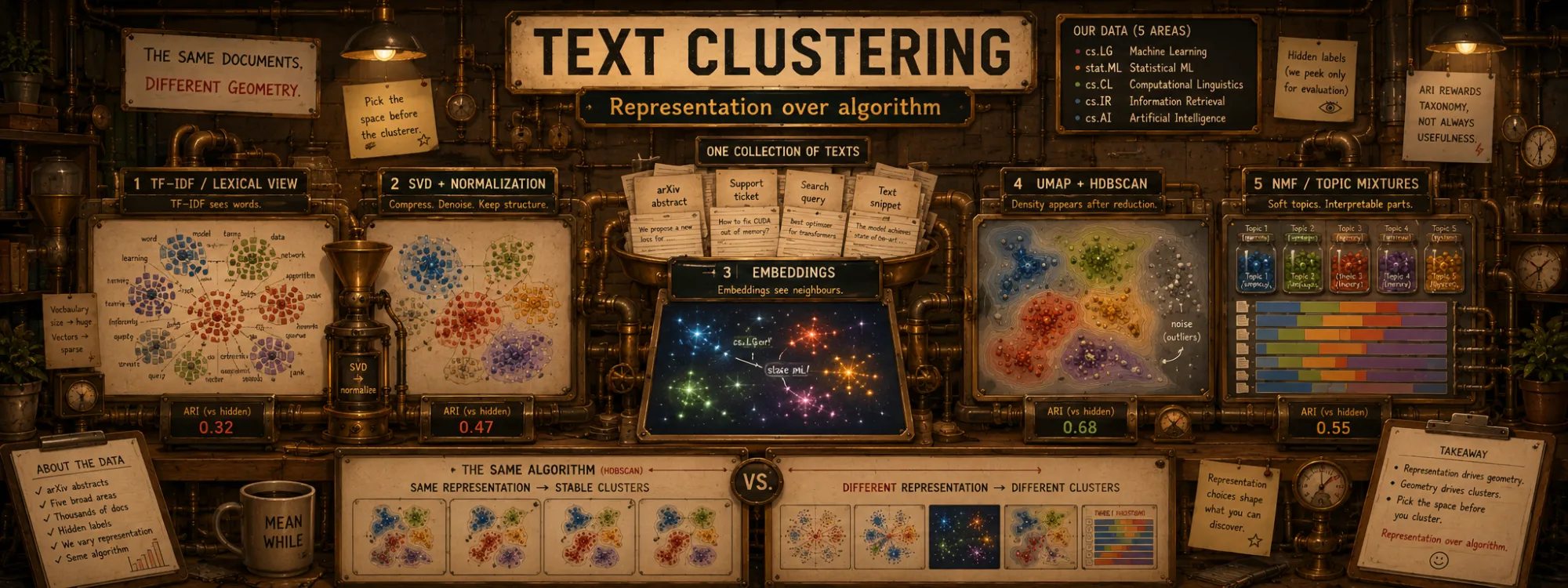
Text Clustering: Representation Over Algorithm
Created Jul 3, 2026 Updated Jul 3, 2026
Read the parent noteThe note’s title is a claim: on real text, the representation you cluster on decides more than the algorithm you pick. But how much more depends on the corpus — so this lab makes the claim visible in two moves. First a controlled case where meaning and surface words are deliberately pulled apart: there the representation decides everything, and no algorithm rescues a bad one. Then the note’s real running example — 550 arXiv abstracts, where the words genuinely carry the meaning — where the representation lever shrinks, and what’s left to separate methods is whether the algorithm matches the geometry. Every number is computed here; no clustering ever sees the labels.
We score every partition against hidden ground-truth labels with the Adjusted Rand Index (ARI) and Normalized Mutual Information (NMI) — 0 for a random grouping, 1 for a perfect match. The conceptual companion — what each method assumes a cluster is — lives in the clustering-methods note.
Requirements
pip install scikit-learn sentence-transformers umap-learn hdbscan numpy pandas matplotlib feedparserNumbers shift a little with a fresh arXiv snapshot or library versions; the finding doesn’t.
Setup
import os, json, time, datetime, urllib.parse, urllib.request
import numpy as np, pandas as pd, torch
import matplotlib.pyplot as plt
from sklearn.feature_extraction.text import TfidfVectorizer
from sklearn.decomposition import TruncatedSVD, NMF
from sklearn.preprocessing import Normalizer
from sklearn.pipeline import make_pipeline
from sklearn.cluster import KMeans, AgglomerativeClustering, SpectralClustering, DBSCAN
from sklearn.mixture import GaussianMixture
from sklearn.neighbors import NearestNeighbors
from sklearn.metrics import adjusted_rand_score, normalized_mutual_info_score
from sentence_transformers import SentenceTransformer
import umap, hdbscan

SEED = 0
np.random.seed(SEED)
# the clustering here is all CPU (scikit-learn); only the E5 embedding step uses a
# GPU when one is around, and just for speed — the numbers are identical either way
device = "cuda" if torch.cuda.is_available() else ("mps" if torch.backends.mps.is_available() else "cpu")
e5 = SentenceTransformer("intfloat/multilingual-e5-base", device=device)   # one embedding model, both experiments

def ari_nmi(pred, true):
    return round(adjusted_rand_score(true, pred), 3), round(normalized_mutual_info_score(true, pred), 3)

print("executed:", datetime.date.today().isoformat())
executed: 2026-07-03Where representation is destiny
The cleanest possible test pulls meaning and surface words apart on purpose. Here are 60 support tickets in four intents — sign-in trouble, a billing dispute, a missing delivery, a cancellation — but each ticket is phrased with different words. Within an intent there is almost no shared vocabulary; across intents the meanings are cleanly separate. A lexical method sees near-random word overlap; an embedding sees four meanings.
groups = {
  "login": ["I can't sign in", "my password won't work", "locked out and can't get in",
            "authentication keeps failing", "the portal rejects my credentials",
            "it says my details are incorrect every time", "two-factor never sends me a code",
            "the reset link in my email does nothing", "it keeps logging me out immediately",
            "my session expires the second I connect", "the app won't let me through the front door",
            "my credentials aren't recognized anymore", "stuck on the verification screen",
            "can't get past the security check on my new phone", "my identity won't validate"],
  "billing": ["I was charged twice for one order", "there is a duplicate transaction on my card",
              "you billed me again this month", "an unexpected fee showed up on my statement",
              "my invoice is higher than the agreed price", "please refund the extra payment",
              "the amount deducted is wrong", "I see two identical debits",
              "my bank shows a repeated withdrawal", "overcharged compared to the quote",
              "the receipt total does not match", "money left my account twice",
              "there is a surcharge I never agreed to", "the plan cost jumped without notice",
              "I want the second charge reversed"],
  "delivery": ["where is my package", "the order has not arrived yet", "tracking shows no movement for days",
               "my parcel is running late", "it was supposed to be here Monday", "the courier never showed up",
               "shipment stuck at the depot", "nothing has been dispatched", "the estimated date keeps slipping",
               "I still have not received my items", "marked delivered but I have nothing",
               "no update since it left the warehouse", "seems lost in transit",
               "when will my goods get here", "the carrier cannot locate my parcel"],
  "cancel": ["I want to cancel my subscription", "please close my account for good", "stop the recurring charge",
             "end my membership immediately", "unsubscribe me from the plan", "I no longer want this service",
             "terminate my contract", "take me off the monthly billing", "shut down my profile permanently",
             "opt me out of renewals", "I would like to discontinue everything", "wind down my account",
             "remove my recurring payment", "I am done, delete my registration", "cease all future charges"],
}
tickets = [t for g in groups.values() for t in g]
t_true = np.array([i for i, g in enumerate(groups.values()) for _ in g])

X_tf = TfidfVectorizer(stop_words="english").fit_transform(tickets)
X_e5 = e5.encode(["query: " + t for t in tickets], normalize_embeddings=True, show_progress_bar=False)

print("cluster 60 paraphrased tickets into 4 intents — same algorithm, two representations:")
for name, run in [("K-means", lambda Z: KMeans(4, n_init=10, random_state=SEED).fit_predict(Z)),
                  ("Agglomerative", lambda Z: AgglomerativeClustering(4).fit_predict(np.asarray(Z.todense()) if hasattr(Z, "todense") else Z))]:
    lt, le = run(X_tf), run(X_e5)
    print(f"  {name:14s}  TF-IDF ARI {ari_nmi(lt, t_true)[0]:.3f}   E5 ARI {ari_nmi(le, t_true)[0]:.3f}")
cluster 60 paraphrased tickets into 4 intents — same algorithm, two representations:
K-means TF-IDF ARI 0.001 E5 ARI 1.000
Agglomerative TF-IDF ARI 0.004 E5 ARI 1.000The lexical representation scores near zero — barely better than shuffling — because the words a customer picks for “I can’t log in” and “authentication keeps failing” overlap almost not at all. The embedding scores a perfect 1.0. And swapping K-means for agglomerative changes nothing: the algorithm is powerless on the wrong representation and unnecessary on the right one. When surface words and meaning diverge, the representation decides everything. That is the thesis in its purest form — now watch what happens on a corpus that sits nearer the other extreme.
A real corpus: 550 arXiv abstracts
Real text is rarely as adversarial as those tickets. Here is the note’s running example: 550 recent arXiv abstracts across five areas, each abstract’s primary category as a hidden label — three clearly distinct (vision, NLP, security) and a deliberately close pair (ML and stats-ML, which share most of their vocabulary). We cache a fixed snapshot so the lab reproduces; the first run pulls a fresh one from arXiv and saves it.
CACHE, CATS = "clustering-corpus.json", ["cs.CV", "cs.CL", "cs.CR", "cs.LG", "stat.ML"]
SHORT = {"cs.CV": "vision", "cs.CL": "NLP", "cs.CR": "security", "cs.LG": "ML", "stat.ML": "stats-ML"}

def fetch_arxiv(cat, want=110):
    import feedparser
    seen, out, start = set(), [], 0
    while len(out) < want and start < 1600:
        q = urllib.parse.urlencode({"search_query": f"cat:{cat}", "start": start, "max_results": 100,
                                    "sortBy": "submittedDate", "sortOrder": "descending"})
        req = urllib.request.Request("http://export.arxiv.org/api/query?" + q, headers={"User-Agent": "lena-notes/1.0"})
        for e in feedparser.parse(urllib.request.urlopen(req, timeout=40).read()).entries:
            if e.get("arxiv_primary_category", {}).get("term") != cat:
                continue
            t = " ".join(e.summary.split())
            if len(t.split()) >= 40 and e.id not in seen:
                seen.add(e.id); out.append(t)
            if len(out) >= want:
                break
        start += 100; time.sleep(3)                            # arXiv etiquette
    return out

if os.path.exists(CACHE):
    with open(CACHE, encoding="utf-8") as f:                    # committed snapshot → reproducible
        data = json.load(f)
else:
    texts, labels = [], []
    for ci, c in enumerate(CATS):
        for t in fetch_arxiv(c): texts.append(t); labels.append(ci)
    order = np.random.RandomState(SEED).permutation(len(texts))
    data = {"names": [SHORT[c] for c in CATS], "labels": [int(labels[i]) for i in order],
            "texts": [texts[i] for i in order]}
    with open(CACHE, "w", encoding="utf-8") as f:
        json.dump(data, f, ensure_ascii=False)

texts, true, names = data["texts"], np.array(data["labels"]), data["names"]
K_TRUE = len(names)
print(f"{len(texts)} arXiv abstracts · {K_TRUE} areas")
for i, nm in enumerate(names):
    print(f"  {nm:9s} {(true == i).sum():>3}")
550 arXiv abstracts · 5 areas
vision 110
NLP 110
security 110
ML 110
stats-ML 110Now the two representations. Lexical: TF-IDF over words, then SVD to 200 dims and L2-normalize — the classic text pipeline. Semantic: the same E5 model, 768-D per abstract. Because the E5 vectors are L2-normalized, Euclidean distance and cosine similarity are monotonic transformations of each other (‖x − y‖² = 2 − 2·cos(x, y)) — so K-means on these embeddings is intentionally close to cosine-style clustering, not an accident.
tfidf = TfidfVectorizer(max_features=20000, stop_words="english", min_df=5).fit(texts)
X_tfidf = tfidf.transform(texts)
lexical = make_pipeline(TruncatedSVD(200, random_state=SEED), Normalizer(copy=False)).fit_transform(X_tfidf)
emb = e5.encode(["passage: " + t for t in texts], normalize_embeddings=True,
                batch_size=32, show_progress_bar=False).astype("float32")
print("lexical (TF-IDF→SVD):", lexical.shape, "  semantic (E5):", emb.shape)
lexical (TF-IDF→SVD): (550, 200) semantic (E5): (550, 768)The representation lever, on lexically-clean text
Repeat the crux experiment — fix K-means, swap the representation:
km_lex = KMeans(K_TRUE, n_init=10, random_state=SEED).fit_predict(lexical)
km_emb = KMeans(K_TRUE, n_init=10, random_state=SEED).fit_predict(emb)
print("K-means, same algorithm, two representations:")
print(f"  lexical  (TF-IDF)  →  ARI {ari_nmi(km_lex, true)[0]:.3f}   NMI {ari_nmi(km_lex, true)[1]:.3f}")
print(f"  semantic (E5)      →  ARI {ari_nmi(km_emb, true)[0]:.3f}   NMI {ari_nmi(km_emb, true)[1]:.3f}")
K-means, same algorithm, two representations:
lexical (TF-IDF) → ARI 0.417 NMI 0.443
semantic (E5) → ARI 0.478 NMI 0.502The embedding still wins — but by a modest margin, nothing like the 0-to-1 chasm on the tickets. That is not a contradiction; it is the finding. Unlike a support ticket, an arXiv abstract wears its topic on its sleeve: vision papers say “segmentation,” security papers say “adversary,” and TF-IDF reads that vocabulary directly. This is exactly the note’s tell in reverse — a sharp jump from TF-IDF to embeddings means the corpus is full of paraphrase and synonymy; a small jump, like here, means the words already are the meaning. The representation lever’s size is a property of the corpus, not the code.
Nine methods, one corpus
The full picture — every sensible pairing, scored against the hidden labels. The density methods cluster on a low-dimensional UMAP projection, because they die on the raw 768-D vectors (next section). One shared UMAP is computed here, for both the density fits and the picture at the end. The goal isn’t to tune each method to its best possible score — it’s to compare reasonable, default-ish pairings on equal footing (spectral or a density method could surely be pushed higher with care).
proj2 = umap.UMAP(n_components=2, n_neighbors=15, min_dist=0.1, metric="cosine",
                  random_state=SEED).fit_transform(emb)                       # 2-D, display only
red5 = umap.UMAP(n_components=5, n_neighbors=15, min_dist=0.0, metric="cosine",
                 random_state=SEED).fit_transform(emb)                        # 5-D, for density methods

agg_lab = AgglomerativeClustering(n_clusters=K_TRUE, linkage="ward").fit_predict(emb)
gmm_lab = GaussianMixture(n_components=K_TRUE, covariance_type="diag", random_state=SEED).fit_predict(emb)
sc_lab = SpectralClustering(n_clusters=K_TRUE, affinity="nearest_neighbors", n_neighbors=15,
                            assign_labels="kmeans", random_state=SEED).fit_predict(emb)
nmf_lab = NMF(n_components=K_TRUE, init="nndsvd", max_iter=600, random_state=SEED).fit_transform(X_tfidf).argmax(1)
hdb_raw = hdbscan.HDBSCAN(min_cluster_size=20).fit_predict(emb)               # raw 768-D
hdb_u5 = hdbscan.HDBSCAN(min_cluster_size=20).fit_predict(red5)               # E5 → UMAP-5
ms = 10
eps = float(np.percentile(NearestNeighbors(n_neighbors=ms).fit(red5).kneighbors(red5)[0][:, -1], 65))
db_lab = DBSCAN(eps=eps, min_samples=ms).fit_predict(red5)

def row(rep, algo, pred):
    a, n = ari_nmi(pred, true)
    return {"representation": rep, "algorithm": algo, "ARI": a, "NMI": n,
            "clusters": len(set(pred.tolist()) - {-1}), "noise%": float(round(100 * np.mean(pred == -1), 1))}

table = pd.DataFrame([
    row("TF-IDF→SVD", "K-means", km_lex),      row("TF-IDF", "NMF (argmax)", nmf_lab),
    row("E5 768-D", "K-means", km_emb),        row("E5 768-D", "Agglomerative", agg_lab),
    row("E5 768-D", "GMM", gmm_lab),           row("E5 768-D", "Spectral", sc_lab),
    row("E5 768-D", "HDBSCAN", hdb_raw),       row("E5→UMAP-5", "HDBSCAN", hdb_u5),
    row("E5→UMAP-5", "DBSCAN", db_lab),
]).sort_values("ARI", ascending=False).reset_index(drop=True)
table| representation | algorithm | ARI | NMI | clusters | noise% | |
|---|---|---|---|---|---|---|
| 0 | E5 768-D | K-means | 0.478 | 0.502 | 5 | 0.0 |
| 1 | E5 768-D | GMM | 0.445 | 0.479 | 5 | 0.0 |
| 2 | TF-IDF→SVD | K-means | 0.417 | 0.443 | 5 | 0.0 |
| 3 | E5 768-D | Spectral | 0.414 | 0.440 | 5 | 0.0 |
| 4 | TF-IDF | NMF (argmax) | 0.359 | 0.390 | 5 | 0.0 |
| 5 | E5 768-D | Agglomerative | 0.358 | 0.388 | 5 | 0.0 |
| 6 | E5→UMAP-5 | DBSCAN | 0.345 | 0.386 | 5 | 6.7 |
| 7 | E5→UMAP-5 | HDBSCAN | 0.173 | 0.258 | 2 | 24.2 |
| 8 | E5 768-D | HDBSCAN | 0.000 | 0.000 | 0 | 100.0 |
Read the ranking honestly. The top line is E5 + K-means — the simplest algorithm on the semantic representation, beating every fancier idea (no discovered k, no noise model, no soft topics, and still first). But on these lexically-clean abstracts, TF-IDF + K-means is right behind it, above two of the embedding methods. What actually sinks a method here is not its representation but an algorithm– geometry mismatch: Ward agglomerative, and (next) HDBSCAN on the raw vectors, fall well below both K-means fits. (Ward is here as a common off-the-shelf hierarchical baseline — it minimizes Euclidean variance, which doesn’t quite match the cosine geometry these embeddings live in, so it isn’t the best possible hierarchical fit for them.) So on real text the shape is: the representation sets a ceiling, and matching the algorithm to the geometry decides who reaches it — with more-flexible methods buying nicer assumptions, not automatically better numbers.
What if we ask for the wrong K?
K-means looks unbeatable partly because we handed it the answer: k = K_TRUE. That is fair for measuring a representation against hidden labels, but a real clustering task rarely knows the number of groups up front. Sweep k and the comfort evaporates:
rows = []
for k in range(2, 11):
    a, n = ari_nmi(KMeans(k, n_init=10, random_state=SEED).fit_predict(emb), true)
    rows.append({"k": k, "ARI": a, "NMI": n})
pd.DataFrame(rows)| k | ARI | NMI | |
|---|---|---|---|
| 0 | 2 | 0.223 | 0.286 |
| 1 | 3 | 0.331 | 0.406 |
| 2 | 4 | 0.488 | 0.502 |
| 3 | 5 | 0.478 | 0.502 |
| 4 | 6 | 0.373 | 0.422 |
| 5 | 7 | 0.430 | 0.479 |
| 6 | 8 | 0.303 | 0.422 |
| 7 | 9 | 0.365 | 0.445 |
| 8 | 10 | 0.258 | 0.403 |
ARI climbs to a broad best around the true k and falls off far from it — ask for too few (k=2 fuses everything) or too many and it shatters. But look closely: the top score sits at k=4, a hair above the true k=5. That is the close pair again — the ML / stats-ML overlap is real enough that merging the two scores marginally better than splitting them, so even the “best” number of clusters here isn’t the true one. Against hidden labels the good range is at least visible; in real exploration, with no labels, choosing k is its own problem (the subject of the clustering-methods note). So “K-means wins” carries an asterisk: it wins given a good k — a gift the benchmark grants and a real task does not.
Where the geometry bites: 768-D vs UMAP-5
The one method that truly collapses is HDBSCAN on the raw embeddings — worth seeing, because it is a representation failure wearing an algorithm’s clothes.
print("HDBSCAN, same algorithm, two geometries:")
print(f"  raw 768-D   →  {row('E5 768-D',  'HDBSCAN', hdb_raw)}")
print(f"  E5 → UMAP-5 →  {row('E5→UMAP-5', 'HDBSCAN', hdb_u5)}")
HDBSCAN, same algorithm, two geometries:
raw 768-D → {'representation': 'E5 768-D', 'algorithm': 'HDBSCAN', 'ARI': 0.0, 'NMI': 0.0, 'clusters': 0, 'noise%': 100.0}
E5 → UMAP-5 → {'representation': 'E5→UMAP-5', 'algorithm': 'HDBSCAN', 'ARI': 0.173, 'NMI': 0.258, 'clusters': 2, 'noise%': 24.2}In high-dimensional embedding space local density is often weakly contrasted: distances compress, neighbourhoods become unstable, and a density-based method struggles to decide what is dense enough to be a cluster — so HDBSCAN finds no clear dense regions and labels almost everything noise. Reduce to 5 dimensions first and the same algorithm, byte for byte, finds structure. HDBSCAN didn’t get smarter; the geometry it saw became more density-friendly. The algorithm was faithfully reporting a geometry the representation had already broken — the note’s point exactly: the algorithm often just formats an error the representation made upstream.
The close pair, and why ARI lies politely
Take the best partition (E5 + K-means) and look at where it agrees with the hidden areas — the contingency table, clusters down, true areas across.
def contingency(pred):
    cl = sorted(set(pred.tolist()) - {-1})
    return pd.DataFrame([[int(((pred == c) & (true == t)).sum()) for t in range(K_TRUE)] for c in cl],
                        index=[f"cluster {c}" for c in cl], columns=names)
contingency(km_emb)| vision | NLP | security | ML | stats-ML | |
|---|---|---|---|---|---|
| cluster 0 | 2 | 3 | 4 | 37 | 71 |
| cluster 1 | 14 | 97 | 9 | 26 | 4 |
| cluster 2 | 1 | 6 | 96 | 6 | 2 |
| cluster 3 | 0 | 3 | 0 | 29 | 31 |
| cluster 4 | 93 | 1 | 1 | 12 | 2 |
The three distinct areas fall into clean, near-pure clusters. The ML / stats-ML pair is the mess — they bleed across the same clusters, because their boundary is partly social and editorial: shared vocabulary, shared methods, many abstracts that could sit in either. No method above solved it. And it is where ARI stops being the whole truth — ARI rewards agreement with the taxonomy, not usefulness. If those two areas are genuinely one intellectual neighbourhood, refusing to split them may be the correct behaviour for exploration, even though ARI punishes it.
The picture
Every method above clustered in full (or reduced) dimension — never on 2-D coords. But a shared 2-D UMAP is a fair display: colour the same points by the hidden areas, then by the winning clustering.
fig, ax = plt.subplots(1, 2, figsize=(7.2, 3.3))
pal = np.array(["#2c5142", "#c4521e", "#3b6ea5", "#b59410", "#7a4fa3"])
ax[0].scatter(proj2[:, 0], proj2[:, 1], c=pal[true], s=6, alpha=.8)
ax[0].set_title("hidden areas", fontsize=9)
ax[1].scatter(proj2[:, 0], proj2[:, 1], c=pal[km_emb % len(pal)], s=6, alpha=.8)
ax[1].set_title("E5 + K-means clusters", fontsize=9)
for a in ax:
    a.set_xticks([]); a.set_yticks([])
plt.tight_layout(); plt.show()
The most useful artefact is the disagreement
A score picks a winner; the disagreement between representations picks the documents worth a human’s eye. Map each K-means partition’s clusters to their majority area, then find the abstracts that land in different areas under lexical vs semantic features — the review pile.
def to_area(pred):                                            # cluster id → its majority hidden area
    m = {c: np.bincount(true[pred == c], minlength=K_TRUE).argmax() for c in set(pred.tolist()) if c != -1}
    return np.array([m.get(c, -1) for c in pred])

lex_area, sem_area = to_area(km_lex), to_area(km_emb)
disagree = np.where(lex_area != sem_area)[0]
print(f"{len(disagree)} abstracts land in different areas under TF-IDF vs E5 — the review pile:\n")
for i in disagree[:3]:
    print(f"  TF-IDF says {names[lex_area[i]]:8s} · E5 says {names[sem_area[i]]:8s} · truly {names[true[i]]}")
    print(f"    {texts[i][:150]}…\n")
179 abstracts land in different areas under TF-IDF vs E5 — the review pile:
TF-IDF says ML · E5 says stats-ML · truly stats-ML
Aqueous solubility is a key property in early-stage drug discovery, but most predictive models merge physicochemical descriptors and molecular graph i…
TF-IDF says vision · E5 says NLP · truly vision
While Multimodal Large Language Models (MLLMs) have advanced video understanding, achieving precise temporal and cross-modal alignment in audiovisual …
TF-IDF says ML · E5 says stats-ML · truly ML
Foundation models are routinely released to the public, yet the data recipes used to train them -- such as domain mixture weights that determine how d…
Those are not errors to hide. A paper the lexical view files one way and the semantic view another is often exactly the cross-cutting work — multimodal LLM work, a foundation-model data recipe, a molecular-prediction paper — that a single clustering would bury. The two representations disagreeing is the signal.
What we just did
We clustered text at two extremes and watched one dial. On paraphrased tickets — meaning and words pulled apart — the representation decided everything: TF-IDF scored ~0, E5 scored a perfect 1.0, and the algorithm was irrelevant in both directions. On real arXiv abstracts — where the words already carry the topic — the same dial barely moved: E5 + K-means still topped the table, but TF-IDF came close, and the real failures were an algorithm–geometry mismatch (HDBSCAN collapsing on 768-D) and an editorial boundary (ML vs stats-ML) that no method, and no representation, resolved. The constant across both: in this lab, the simplest pairing — embeddings + K-means — was never beaten by something fancier (and even that came with an asterisk: it was handed the right k). Choosing the representation isn’t preprocessing — it sets the ceiling on how much the algorithm can even matter, and how high that ceiling sits is a fact about your corpus.