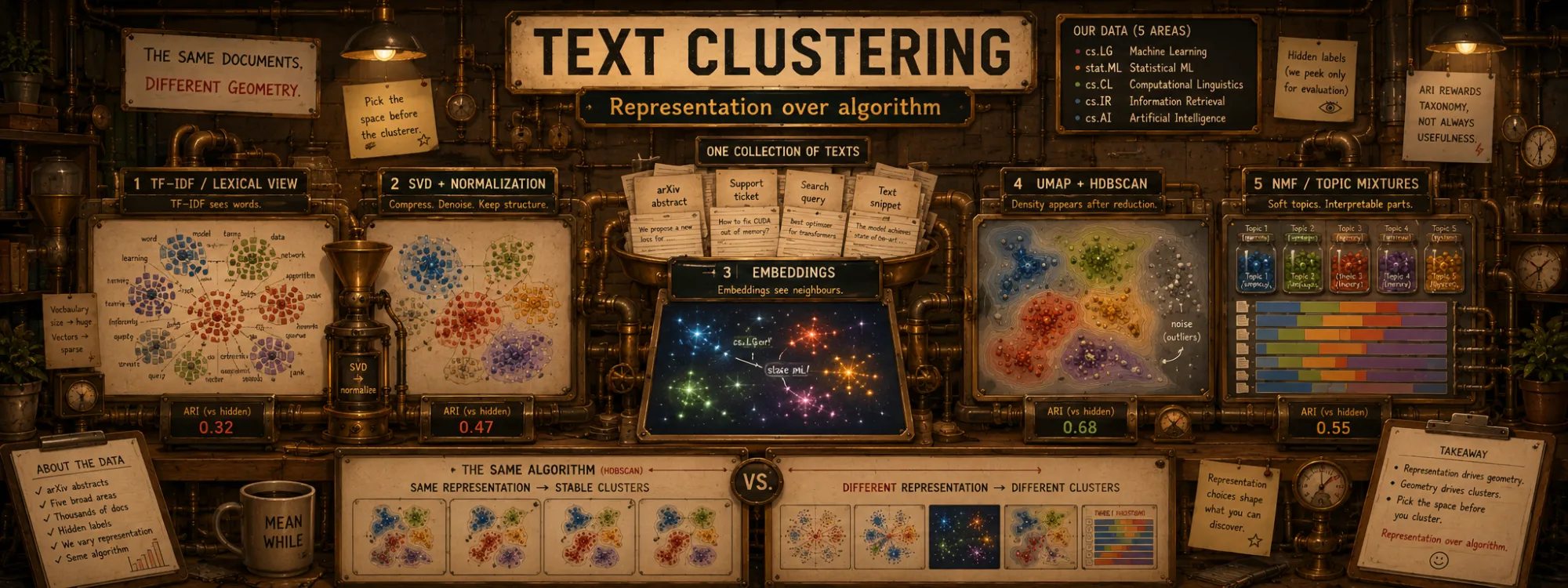
Text Clustering: Representation Over Algorithm

Clustering text — support tickets, search queries, a pile of abstracts — feels like a question of which algorithm to pick. On real text it usually isn't: the thing that moves the result most is the representation you cluster on (bag-of-words, TF-IDF, or learned embeddings), and the algorithm is often a footnote next to that choice.

The effect is easiest to see where surface words and meaning are deliberately pulled apart. Take 60 support tickets across four intents — sign-in trouble, a billing dispute, a missing delivery, a cancellation — each written with different words, so within an intent the vocabulary barely overlaps. A lexical representation sees near-random word overlap; an embedding sees four meanings. Run the same K-means on each:

That is the thesis in its purest form — the representation decides everything, and no algorithm rescues a bad one. Real corpora are rarely so adversarial, and the size of the effect shrinks the more the surface words already are the meaning. So the rest of this note runs the same comparison on a harder, more realistic case: one shared corpus of 550 recent arXiv abstracts across five areas — three clearly distinct (computer vision cs.CV, NLP cs.CL, security cs.CR) and a deliberately close pair (machine learning cs.LG and statistics-ML stat.ML, which share most of their vocabulary). Each abstract's true area is its primary arXiv category, so every clustering can be scored against ground truth with the Adjusted Rand Index (ARI) — but no algorithm ever sees the labels. Here the topical vocabulary is distinctive enough that TF-IDF reads much of it directly, so the representation lever is real but far more modest than on the tickets. The widgets below are real fits; every number is read off an actual run (scripts/compute_clustering_example.py), and a runnable companion lab reproduces the whole comparison end to end.

The geometry of each method — what it assumes a cluster is — lives in a separate note, clustering methods. This one is about what happens when you point them all at the same text.

---

Experiment setup

The corpus is intentionally small enough to inspect and large enough for the algorithms to stop behaving like toys: 550 recent arXiv abstracts, 110 per area, sampled across cs.CV, cs.CL, cs.CR, cs.LG and stat.ML, with headers, footers and quote blocks stripped. The label is each paper's primary arXiv category, used only after fitting to compute ARI and NMI.

For the lexical baseline I use TF-IDF (max_features=20000, min_df=5, English stop-words), then TruncatedSVD to 200 dimensions to densify and denoise, then L2 normalisation before K-means (n_init=10). The embedding runs use E5 sentence vectors (intfloat/multilingual-e5-base, each abstract prefixed with passage: and L2-normalised on output — the multilingual variant is just the embedder I had on hand; the corpus itself is English, which is also why the TF-IDF stop-words are English). The density runs compare the raw 768-D embeddings against a UMAP-reduced space (n_components=5, n_neighbors=15, min_dist=0.0, cosine metric), because HDBSCAN usually needs a lower-dimensional space where density gaps are visible. The 2-D scatter in every widget is a separate, display-only UMAP (min_dist=0.1); clustering never happens on those two coordinates. Everything runs at random_state=0.

The point is not to declare a universal winner. It is to keep the corpus fixed and watch what changes when only the representation and the clustering assumptions change.

---

The classic baseline: TF-IDF → SVD → Normalizer → KMeans

Naive K-means on raw TF-IDF gives bad clusters: with tens of thousands of sparse features the distances stop meaning much and the centroids become diffuse averages over many rare words. The fix is a four-step pipeline that turns K-means into a perfectly serviceable document-clustering baseline — the standard classical recipe in the scikit-learn ecosystem:

1. TF-IDF. Build a sparse document × word matrix; the dimensionality is the vocabulary size, usually tens of thousands.
2. TruncatedSVD (also called LSA — Latent Semantic Analysis). Reduce to 100–300 dimensions. This is the step that breaks the curse of dimensionality and removes noise from rare words.
3. Normalizer. Scale every vector to unit L2 norm. For two individual normalised documents, Euclidean distance is then monotonically equivalent to cosine distance — ‖x − y‖² = 2 − 2·cos(x, y) — which is why this pipeline behaves like a cosine-based clustering baseline in practice. (It is an approximation, not exact spherical K-means: the centroids themselves are not re-normalised after each update.)
4. KMeans. Ordinary K-means on the resulting dense 100–300-dimensional representation.

from sklearn.feature_extraction.text import TfidfVectorizer
from sklearn.decomposition import TruncatedSVD
from sklearn.preprocessing import Normalizer
from sklearn.cluster import KMeans
from sklearn.pipeline import Pipeline

pipeline = Pipeline([
    ("tfidf", TfidfVectorizer(max_features=20000, min_df=5, stop_words="english")),
    ("svd", TruncatedSVD(n_components=200)),
    ("norm", Normalizer()),
    ("kmeans", KMeans(n_clusters=10, n_init=10)),
])
pipeline.fit(documents)

SVD compresses and densifies; L2 normalisation makes the distance behave like a cosine-based comparison between documents. What this pipeline does not fix is synonymy and paraphrase: "refund not received" and "my money hasn't come back yet" are nearly different documents to TF-IDF. So it is the right choice for longer, cleaner texts (articles, documents, detailed tickets) in a narrow domain with predictable vocabulary, and the wrong choice for short paraphrased text, multilingual data, or noisy user-generated content — where embeddings earn their keep.

I expected the embedding run to win, but not by this much. The algorithm did not change, K did not change, and the labels were still hidden — only the representation changed, and ARI moved from 0.36 to 0.51. That is the moment this stopped being a clustering-method comparison and quietly became a representation comparison.

---

What the representations see

TF-IDF sees vocabulary. It is good when the language is stable and domain-specific: if security papers repeatedly say memory, attack, privacy, exploit, the lexical signal alone is enough. It is bad when two texts mean the same thing in different words, or when one theme is written in several languages or styles.

Embeddings see semantic proximity. They pull together paraphrases and related concepts, which is why the same K-means improves when the input changes from the TF-IDF pipeline to E5 vectors. But embeddings are not magic labels: if two fields genuinely share methods and vocabulary — as cs.LG and stat.ML do — the embedding space may correctly place them near each other, even when the taxonomy wants them apart.

UMAP changes the question again. It is not just compression; it reshapes the neighbourhood graph. That can make density visible for HDBSCAN, but it can also turn a continuous field into a few coarse basins — which is why the reduced HDBSCAN run looks alive while the raw one collapses, and still does not recover the five arXiv labels.

---

Soft topics, not hard buckets: NMF

Strictly speaking, NMF is not a clustering algorithm in the same sense as K-means — it is a matrix-factorisation / topic-modelling method. It belongs in a text-clustering note because it is so often used inside these workflows: it produces soft document–topic assignments and an interpretable low-dimensional space to group documents in. It was proposed by Paatero and Tapper in 1994 and popularised by Lee & Seung in 1999, and its distinguishing property is a non-negativity constraint on every value in the decomposition, which keeps the result far more interpretable than SVD or PCA, where components can be negative and lose clear meaning.

The idea

Decompose matrix X into the product W × H where every value is ≥ 0:

X[docs × words]  ≈  W[docs × topics] × H[topics × words]

X is the (sparse) document-word matrix with TF-IDF weights; W (docs × K) and H (K × words) are the factors. K is the chosen number of topics, usually 5–100. Effectively: "the document-word matrix is a linear combination of K basis topics, where W tells which topics each document belongs to and H tells which words characterise each topic."

The interpretation is clean. W[i, :] is the profile of document i in topic space — e.g. [0.8, 0.0, 0.2, 0.0, …] says the document is 80% topic 0, 20% topic 2, nothing else. H[k, :] is the set of words for topic k — high values for revenue, quarter, earnings on a financial topic; high values for server, deployment, bug, pipeline on an IT topic. You look at the top words of each topic, name it, and work with meaningful categories instead of opaque cluster IDs.

Optimisation

NMF is the constrained optimisation problem:

minimise  ‖X − WH‖²    subject to  W, H ≥ 0

The problem is non-convex, so there is no global solution — only local optima. The reconstruction loss is most often the Frobenius norm shown above, but a Kullback–Leibler-divergence variant exists too (especially natural for count-style data); scikit-learn exposes both via the beta_loss parameter. Two training algorithms are in classical use: multiplicative updates (the original Lee–Seung 1999 algorithm) and coordinate descent, the latter usually faster on sparse data and the scikit-learn default.

What NMF buys, and how it differs from K-means

Three things make NMF worth the trouble. It is soft: a document can belong to several topics in proportions, a far more realistic model of text than forcing each one into a single bucket, since a question can touch several themes at once. It is interpretable, because H reads off directly as "topic = a set of words"; where a 768-dimensional BERT embedding is an opaque vector with no per-dimension meaning, NMF hands you explicit topic-word semantics you can name. And the non-negativity is not just a technicality. With no cancellation allowed (a word cannot occur "minus three times" in a topic), documents come out as sums of positive parts, and that is what keeps the result legible.

The common misconception is that NMF "replaces K-means for sparse data". Not quite — they answer different questions. K-means gives a hard partition: each document falls into exactly one cluster ("into what groups is my data divided?"). NMF gives a soft mixture: each document is a blend of K topics ("what topics are hidden in my corpus and how are they mixed in each document?"). "Group these 10 000 tickets into 8 buckets for 8 teams" is K-means; "show me the main topics in a corpus and how they evolve" is NMF or LDA.

When you want both interpretability and a hard partition, the two compose: run NMF first as interpretable dimensionality reduction, then K-means on the topic matrix W.

from sklearn.decomposition import NMF
from sklearn.cluster import KMeans

nmf = NMF(n_components=50, init="nndsvd", max_iter=500)
W = nmf.fit_transform(X_tfidf)        # (docs × 50 topics), dense, non-negative

kmeans = KMeans(n_clusters=8, n_init=10)
labels = kmeans.fit_predict(W)

The 50-dimensional topic space replaces the 20 000-dimensional word space, each axis carries meaning via H, and the K-means clusters can then be explained through "which topics dominate at the centroid". The trade-off against the SVD pipeline above: SVD gives a mathematically optimal low-rank approximation with uninterpretable axes; NMF gives interpretable topics at the cost of a less-optimal reconstruction.

In practice, init="nndsvd" (Non-negative Double SVD) beats random initialisation, especially on sparse data, and the scikit-learn default of max_iter=200 is often too few for complex corpora.

What I actually reach for here is the right-hand column. A paper that comes out 40% one topic and 30% another is usually the interesting one: the cross-over work that a hard label would flatten into a single bucket and quietly hide. The mixed examples are not always semantically clean, though — sometimes the split exposes topic leakage or an imperfect factor rather than genuine cross-over work, which is exactly why I read them instead of trusting W as ground truth.

---

Embeddings, UMAP, HDBSCAN — the BERTopic recipe

The modern default for messy short text is to drop TF-IDF entirely: embed each document with a sentence model, optionally reduce with UMAP, cluster the result with HDBSCAN, and label the clusters with c-TF-IDF. That combination — embeddings + UMAP + HDBSCAN + c-TF-IDF — is exactly BERTopic, the recipe many people reach for first when they need topic-like clusters out of messy text without committing to a K up front. HDBSCAN earns its place here because it needs no K, separates noise into an explicit -1 label, and tolerates clusters of uneven size — the typical shape of real chat logs, search queries, and reviews.

This corpus is HDBSCAN's hard case: long, homogeneous abstracts that are all "ML papers", with no real density gaps between the areas. On the raw 768-D vectors it collapses to all-noise; even with the UMAP step it finds only a couple of coarse basins. Its strength is the opposite kind of data — well-separated groups of uneven density sitting in a field of noise — and there is a toy of exactly that case in clustering methods. Here, the one thing it does that K-means cannot — decline to assign a point — is not what the data needed.

---

Nine methods, one corpus

The annoying thing about K-means is that it is often good enough. On this corpus, embedding + K-means is not elegant — it does not discover K, does not model noise, and does not produce soft topic mixtures — and yet it is still the highest-scoring clustering in the whole comparison. That is a useful embarrassment: more flexible methods buy you nicer assumptions, not automatically better results.

None of the other fits is wrong, exactly. Each one fails in a way that tells you what it can see:

1. TF-IDF + K-means separated security cleanly, but blurred the cs.LG / stat.ML boundary.
2. E5 + K-means lifted the global score, yet still did not solve the close-pair problem.
3. Raw-embedding HDBSCAN found no hidden structure at all — it labelled everything as noise.
4. UMAP + HDBSCAN recovered density, but only as a couple of coarse basins, not the five areas.

Each failure is the method telling us what kind of structure it is able to see.

The close pair is the real trap here. cs.LG and stat.ML are not badly separated because the algorithms are weak — they are badly separated because the boundary is partly social and editorial: the vocabulary overlaps, the methods overlap, and many abstracts could plausibly live in either category. This is exactly where I would stop treating ARI as the whole truth. ARI is useful only because arXiv hands us hidden labels to compare against, but it lies politely — it rewards agreement with the taxonomy, not usefulness. If cs.LG and stat.ML are genuinely overlapping intellectual neighbourhoods, then failing to split them cleanly may be the correct behaviour for exploration, even though ARI punishes it.

And the most useful artefact is often not the best clustering but the disagreement between clusterings. A document that is "security" under TF-IDF and "NLP" under embeddings may be a paper on LLM watermarking; a document K-means assigns confidently but HDBSCAN marks as noise may be lexically close to a theme without sitting inside a dense semantic region. These are not errors to hide — they are the review candidates worth a human's attention.

---

How I would review the result

A clustering score is only the first filter. After it, I inspect each cluster through four views: the top c-TF-IDF words, a few medoid documents, a few borderline documents, and the confusion against whatever labels I happen to have.

The medoid tells me what the cluster is centred on. The top words tell me how I might name it. The borderline examples tell me where it leaks into a neighbouring theme. The confusion matrix tells me whether I am recovering an existing taxonomy or discovering a different structure.

That last distinction matters. If the goal is to reproduce an existing routing scheme, disagreement with the labels is bad. If the goal is exploration, disagreement may be the whole point.

---

The two mistakes are not symmetric

In text clustering, false merges and false splits hurt differently.

A false merge puts two different themes in one bucket. This is what happens when cs.LG and stat.ML collapse together: the cluster may still be intellectually coherent, but it stops matching the taxonomy. For exploration that may be fine; for routing papers to reviewers or tickets to teams, it is a problem.

A false split breaks one theme across several buckets. This is what lexical methods do to paraphrase: "cannot log in" and "password reset isn't working" can land far apart even though the action they need is identical.

The right representation depends on which mistake is more expensive. TF-IDF tends to split paraphrases; embeddings tend to merge neighbouring concepts. That is why choosing the representation is not a preprocessing detail — it is a product decision.

---

What I would run first in a real project

For a real text-clustering task I would start with two deliberately boring baselines.

First, TF-IDF → SVD → Normalizer → K-means. It is cheap, reproducible, easy to explain, and gives a lexical view of the corpus. If it finds clean groups, those groups are driven by words people actually use — which is often exactly what an operations team cares about.

Second, embeddings → K-means, with K taken from the business question rather than from the metric alone. If the result improves sharply over TF-IDF, the corpus probably contains paraphrase, synonymy, or semantic groupings that lexical features miss.

Only then would I reach for embeddings → UMAP → HDBSCAN — not because it is more fashionable, but because it answers a different question: are there dense semantic regions and a meaningful long tail of noise? If HDBSCAN marks many points as noise, I do not treat that as failure by default. I read the noise. Sometimes it is garbage; sometimes it is the new work.

---

What I would not reach for first

I would not start with spectral clustering on 50,000 support tickets unless I had a specific reason to believe the similarity graph hides non-convex structure worth preserving. I would not start with GMM on raw 768-dimensional embeddings unless I had already reduced the space and actually cared about probabilistic responsibilities. And I would not start with raw HDBSCAN on long, homogeneous scientific abstracts expecting clean topical categories to fall out — this experiment already showed how that ends.

When the clustering looks wrong

When a partition comes out bad, I debug in roughly this order:

1. Look at the representation before blaming the clusterer.
2. Check whether the labels you expect are even separable in this space.
3. Inspect the nearest neighbours of a few points from each confused class.
4. Put a lexical (TF-IDF) and an embedding-based clustering side by side.
5. Treat HDBSCAN's noise as signal, not garbage.
6. Read the borderline examples before touching any parameters.

One caveat on how far this generalises: the corpus is not representative of all text clustering. It is deliberately clean, long-form, technical and English — not support tickets, search queries or chat logs. On short or multilingual messages the relative behaviour can shift: lexical baselines often break harder, while HDBSCAN can become genuinely useful, because there the long tail and the noise are real. And what stumbled here was not HDBSCAN as a method — it was a mismatch between a density-seeking algorithm and a continuous academic-topic manifold with no density gaps to find.

The lesson is not that embeddings always win, or that K-means is secretly the best algorithm. It is narrower and more useful: in text clustering, the representation decides what kinds of mistakes the system will make, and the clusterer only formalises those mistakes into labels.

Once the clusters look right, naming and validating them is a separate job — labelling, two-corpus comparison, choosing K, and the standard mistakes are covered in clustering in practice.