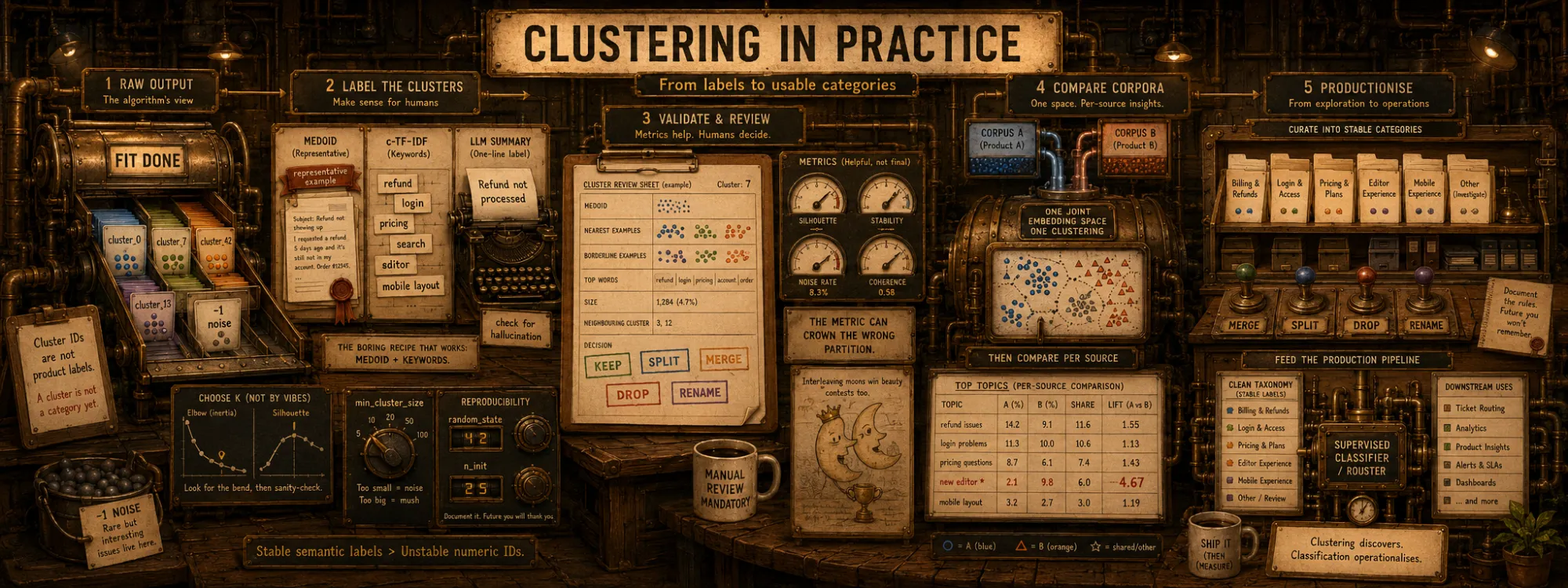
Clustering in Practice

Picking a clustering algorithm is only the first step. After fitting comes a series of practical questions: how to describe each cluster to a human, how to compare two corpora through the same partition, how to validate that the result is meaningful, which parameters to turn first when something looks wrong, and what makes the partition reproducible across runs. None of these are about the algorithms themselves; they are about working with the results.

This note is the applied wrap-up to the clustering methods and text clustering notes. It assumes the algorithm has been chosen and the data is in a clusterable shape.

---

A cluster is not a category yet

The algorithm gives you integer labels. A product needs categories. The gap between the two is not cosmetic: a cluster can be statistically tight and still useless, or messy but operationally meaningful. Before a cluster becomes a category it has to survive three checks — can a human name it, can another human recognise it, and does the name imply a useful action? Everything below is about getting clusters across that gap.

---

Cluster labelling

A cluster is just a number assigned to a group of points. To make it useful to a person, it has to be described in words. This is a separate task, applicable to any clustering algorithm; in text clustering specifically, there are three standard techniques of varying complexity (the keyword-extraction technique below is text-specific; the others generalise to any data with a notion of similarity).

Medoid — a real representative

The simplest and most robust labelling is to pick a medoid. Strictly, the medoid is the real point with the smallest average distance to the other points in the cluster; in practice, for large clusters, a cheaper approximation is the point closest to the centroid. Unlike the centroid, which is just a point in vector space without a direct human reading, the medoid is a real text from the original data. It can be shown to the user as a "typical example of this cluster" and is immediately understandable.

Computationally: for a cluster of n points, compute the n × n matrix of pairwise cosine similarities; for each point sum its similarities to all other points in the cluster; take the point with the maximum sum. The same idea is the basis of K-medoids (PAM) — except K-medoids uses medoids as cluster centres throughout the algorithm, while for labelling we only need the final selection.

The strong side of the medoid is zero risk of hallucination — a real text from the data is shown, no rewriting. The weak side is that the medoid may be long, contain a corner case, or fail to capture the breadth of a diverse cluster. For broad clusters, showing N points closest to the medoid as "extended examples" supplements the single-medoid view.

c-TF-IDF — keywords of the cluster

c-TF-IDF (class-based TF-IDF) is a generalisation of classical TF-IDF popularised by the BERTopic library. The idea: glue all texts in one cluster into a single "macro-document", treat the clusters as a corpus, and run TF-IDF on this corpus. The top-N words by c-TF-IDF score for each cluster are the words that occur often in this cluster but rarely in others — i.e. the discriminative keywords of the topic.

Where classical TF-IDF gives keywords of an individual document, c-TF-IDF gives keywords of a topic. Including bigrams (ngram_range=(1, 2)) helps because many topics are described better by stable phrases than by single words.

The strong side is compact, discriminative keys: five words usually let a person grasp the topic boundaries instantly. The weak side is that the keywords do not form a natural sentence, and for languages with rich morphology (Russian, German, Finnish) it pays to lemmatise first, otherwise different forms of the same word compete for the top.

LLM summarisation — flexible but expensive

The third technique is to ask an LLM to generate a one-sentence description of the cluster from a few examples. The quality is usually higher than medoid + keywords — the model can catch nuances that neither captures (cluster of subjunctive-mood questions, cluster of complaints in a specific tone).

The cost: an LLM call per cluster (latency, money) and a hallucination surface (the model may describe the cluster as something it is not, especially when borderline points are in the sample). The risk has to be either accepted in the workflow or reduced through careful prompting and a curated sample (e.g. only the medoid plus a few nearest points).

The boring recipe that works surprisingly often

For most tasks, medoid + top-N c-TF-IDF words is enough. The medoid gives the "face" of the cluster — a concrete example that reads instantly; c-TF-IDF gives the thematic key that makes the boundaries between topics visible. Both are cheap compared with LLM summarisation, introduce no generative step (so no hallucination risk), and are easy to implement on standard scikit-learn tools. LLM summarisation is worth adding only when there is a concrete signal that medoid + words is not enough for the target reader.

This recipe is universal across algorithms. K-means gives a centroid but not text — the medoid restores the text. NMF gives word distributions via the matrix H — c-TF-IDF on the documents of each cluster usually produces a comparable human-readable explanation and works the same way for embedding-based clusters where H does not exist. HDBSCAN gives neither by construction — these techniques fill the gap.

---

Comparing two corpora through a unified embedding space

A separate class of problems is not "find structure in one corpus" but compare the structure of two corpora. Examples: drift detection (has the distribution of texts changed between period A and period B?), comparing product versions (which topics appear in the new version's user feedback that didn't appear before?), measuring topic intersection between two sources. Two approaches with very different diagnostic value:

What does not work: independent clustering of each corpus

The first intuition is to cluster each corpus separately, get two sets of clusters, and compare them by pairwise similarity of centroids or medoids. This sounds natural ("first understand each, then compare") but in practice produces mostly artefacts:

• Two independent runs of any clustering algorithm — especially HDBSCAN or K-means with different K — produce different partitions of the same kind of data. A topic that formed one cluster in corpus A may split into three in corpus B, or merge with a neighbour. Matching these heterogeneous groups directly is incoherent.
• The metric "how similar is cluster A to cluster B" reduces to an argument about a threshold: at what cosine similarity between medoids should a pair count as "the same topic"? Any choice of threshold leaves a band of borderline pairs that one method calls a match and another does not. There is no substantive answer.
• Each independent run produces its own noise, and the noises do not have a shared semantic basis to be compared.

What works: joint clustering with per-source counts

For exploratory comparison, the safer default is to cluster the union of the two corpora in one run, tagging each point with the source it came from. The output is a single shared set of clusters (the same topics for both corpora), and each topic is characterised by a pair of counts: how many points of this topic came from corpus A and how many from corpus B.

This gives direct answers to substantive questions. Topics with large counts on both sides are common to both. Topics with a large A count and zero B are present only in A. Topics with the opposite pattern are unique to B. Topics with asymmetric counts (100 vs 5) are present in both with different intensity, often a useful signal.

Raw counts are not enough, though. A topic with 100 items is huge in a 1,000-item corpus and tiny in a 1,000,000-item one. For comparison, report both counts and shares, then sort by lift — share_B / share_A. The high-lift topics are usually where regressions, new user pain, or emerging themes show up. Never sort by lift alone, though: apply a minimum count threshold or smoothing to the denominator, otherwise a topic going from 1 item to 5 shows up as a 5× explosion and drowns the real signals.

There is also a sampling trap: if one corpus is much larger, it can dominate the joint clustering geometry and the discovered topics will reflect the big corpus. In that case, cluster a balanced sample for discovery, then assign the remaining points to the discovered clusters — or at the very least report shares rather than raw counts.

The advantage is a unified embedding space and a unified partition. Any point from A and any point from B are evaluated by the same distance metric and assigned under the same distance geometry, so a shared cluster has a clear interpretation: the algorithm grouped them as semantically close in the same sense for both corpora. No threshold, no matching, no artefacts of different runs.

The clustering is usually HDBSCAN, because the number of common topics is unknown in advance and noise of different nature is correctly separated in both corpora at once. The visualisation is naturally complemented by a UMAP projection coloured by cluster and with an additional marker by source (different point shape or symbol) — both the thematic structure and the per-source distribution are then visible at once. As a conservative default, cluster on the full embeddings and use UMAP only for display. If you use a BERTopic-style UMAP → HDBSCAN pipeline instead, treat UMAP as part of the model — tune it deliberately and validate it — and do not confuse that reduced clustering space with the 2-D projection you draw.

This is the right default for a one-off comparison. For recurring monitoring it has a cost: reclustering the union from scratch every period reshuffles the taxonomy, so period-over-period categories stop lining up. Once the categories are curated, a fixed classifier — or assigning new points to a set of reference clusters — is usually better than reclustering each time (the clusters-to-categories section covers the pattern).

The applicability has one limitation: both corpora must be representable in a unified embedding space. If they are in different languages, a multilingual embedding model is needed; if they are in completely different domains (scientific articles vs tweets), the common clusters may be too abstract to be useful, and pre-filtering both corpora to a narrower common scope is the workaround.

---

Validating clustering quality

Clustering is a task without ground truth, and validating the result is itself a non-trivial problem. Three parallel approaches — none self-sufficient, in production they are usually combined.

Internal metrics

Numerical evaluations based on the data alone, without external labels. They look at how compact clusters are inside and how separated they are between each other.

• Silhouette score — for each point, s = (b − a) / max(a, b) where a is mean distance to points in its own cluster and b is mean distance to points in the nearest neighbouring cluster. Range [-1, 1]: positive = the point fits its cluster, around zero = on the boundary, negative = probably misclassified. The metric is the average s over all points. Intuitive interpretation; exact computation is effectively quadratic on large corpora, so in practice it is often computed on a sample.
• Davies–Bouldin index — ratio of within-cluster spread to between-cluster distance, averaged over pairs of clusters. Lower is better, ideal around 0. Does not require pairwise distances and is O(N·K).
• Calinski–Harabasz index (variance ratio) — ratio of between-cluster variance to within-cluster variance. Higher is better. Fast to compute, well-correlated with intuitive quality.

All three are useful for comparing different parameters of the same algorithm (choosing K in K-means via silhouette on a grid). For comparing different algorithms, they are less reliable: they implicitly prefer a particular cluster geometry (sphere-like), so an algorithm that produces precisely that shape (K-means) systematically wins over algorithms looking for arbitrary shapes (HDBSCAN), even when the latter are semantically more correct.

Topic coherence — for topic modelling

If the task is topic extraction (NMF, LDA, BERTopic), the standard metric is coherence between the top words of each topic. The intuition: good top words tend to co-occur in the same documents. Several variants:

• C_V — combines NPMI with cosine similarity between context vectors over a sliding window; the most popular variant.
• U_Mass — log of the conditional probability of words co-occurring in documents.
• C_UCI — PMI on a sliding window.

Different variants sometimes give different rankings, so academic papers typically report several. Coherence is meaningful for topic models specifically, not for arbitrary clustering.

Stability — robustness to perturbations

A useful practical signal: run the algorithm two or three times on the same data with different random seeds (or on bootstrap samples) and compare the results via Adjusted Rand Index (ARI) or Normalized Mutual Information (NMI). High stability (e.g. ARI > 0.8) is a strong signal that the partition is not just an artefact of random initialisation, though it does not by itself prove the clusters are semantically useful — stable nonsense exists too, especially when preprocessing is grouping points by surface features (text length, request framing) rather than topic. Low stability means the K-group partition is forced, and a different K or algorithm should be tried. For production systems where clustering is retrained on fresh data periodically, stability is critical: unstable clustering produces "jumping" cluster IDs and downstream logic that depends on those IDs breaks.

Manual review — the mandatory check

No numerical metric replaces opening a random sample of clusters and reading the examples. Concretely: for 5–10 randomly chosen clusters, look at the medoid plus 5–10 nearest points and ask — does this look like a meaningful topic? Is the cluster picking up something singular, or is it a mixture? Is it clear how this cluster differs from neighbouring ones? If clusters do not look meaningful by eye, no silhouette score will save the result. Even a 30–60 minute manual review on a moderate corpus often gives an order of magnitude more understanding than any numerical score.

A useful structure is a per-cluster review sheet. For each cluster, look at:

• the medoid;
• its 5 nearest examples;
• 5 borderline examples (lowest membership, nearest the boundary);
• the top c-TF-IDF words;
• its size and any noise-adjacent points;
• the nearest neighbouring cluster;
• and a decision: keep / split / merge / drop / rename.

The decisions carry specific meanings. Keep — the cluster is coherent and useful. Split — it holds two distinct actions under one surface theme. Merge — the algorithm separated variants that humans treat as the same issue. Drop — it is boilerplate, garbage, or simply not actionable. Rename — the cluster is real but the automatic label is misleading.

For K-means, silhouette is a reasonable parameter-selection tool. For HDBSCAN it is only a weak diagnostic, usually computed after setting the noise aside — there, the noise rate, cluster stability, HDBSCAN's own validity score (DBCV), and manual review matter far more than maximising silhouette. So the practical formula differs by method:

• K-means: silhouette → stability → eyes.
• HDBSCAN: noise rate → stability / validity → eyes.

---

Choosing K when it isn't known

K-means, GMM, NMF, LDA and fixed-count Agglomerative all need K up front. When the problem doesn't hand it to you, there is no ground truth and no formally optimal K — only a small toolkit of heuristics, each with its own failure mode.

Elbow rule

The classic heuristic. Plot inertia (sum of squared distances to each point's centroid) against K; it falls monotonically, and the "elbow" — where the drop suddenly flattens — is your K:

inertias = [KMeans(n_clusters=k, n_init=10).fit(X).inertia_ for k in range(1, 20)]
plt.plot(range(1, 20), inertias)

Beyond the natural K, extra clusters only carve up already-good ones — that is the theory. In practice the bend is often ambiguous or absent, so treat the elbow as a sanity check, not an answer.

Silhouette score on a grid

More discriminating: compute the average silhouette (defined in "Internal metrics" above) at each K and take the maximum — a number, not a visual judgement.

The catch: silhouette favours sphere-like clusters, so on non-spherical structure it can systematically pick the wrong K. Trust it on K-means-shaped data; cross-check it on anything else.

Gap statistic

The formal version of the elbow (Tibshirani, Walther & Hastie, 2001): compare within-cluster dispersion at each K against a null reference (uniform random data over the same range), and take the smallest K whose gap beats the null by more than one standard error.

A principled stopping rule, but it samples the null distribution and costs more than silhouette. In libraries like gap-statistic (OptimalK), not scikit-learn directly.

Stability-based selection

A different angle: a real K survives perturbation. Cluster bootstrap samples at each candidate K, take the average pairwise Adjusted Rand Index (ARI) between runs, and prefer the most stable K.

If K is right, bootstraps return the same clusters; if it is too high, the forced splits reshuffle between runs. It costs more than silhouette but fails differently — the two together beat either alone.

Information criteria for probabilistic models

For likelihood-based models, formal model-selection criteria are available:

• BIC / AIC for GMM — penalise log-likelihood by parameter count. Lower is better.
• Perplexity for LDA — held-out negative log-likelihood per token. Lower is better.

Better grounded than the heuristics above, but only for probabilistic models — not plain K-means or hard NMF.

A practical recipe

No single method gives a defensible K on its own. The sweep I actually run:

1. Run K-means on a grid K ∈ {3, 5, 8, 10, 15, 20, 30, 50}.
2. Compute silhouette for each K and plot.
3. Compute stability (average ARI across 10 bootstraps) for each K and plot.
4. Take the top 2–3 candidates and manually review the resulting clusterings — open the medoids and a few sample points per cluster, see which K produces the most semantically meaningful partition.

Numbers narrow eight candidates to two or three; eyes pick between those. A sharp disagreement between silhouette and stability is itself a signal that the data may have no natural K — worth a switch to HDBSCAN (no K) or topic modelling (mixture, not partition).

In practice I rarely expect the K-selection plot to answer the question — I expect it to eliminate the bad choices. If K = 5 and K = 8 both look plausible numerically, the real decision is usually operational: how many categories can the downstream team actually use?

If the algorithm doesn't require K at all — HDBSCAN, DBSCAN, BERTopic — the choice has been delegated to a different parameter (min_cluster_size), and the corresponding entry in the next section covers how to set it.

---

---

Hyperparameter tuning order

When the first run gives a bad result, turning parameters in the right order avoids combinatorial drift and pinpoints the real cause. The order matters because tuning clustering is otherwise a perfect way to fool yourself: change K, preprocessing, embedding model, UMAP, and min_cluster_size all at once and you no longer know what fixed the result.

K-means. Main parameter: n_clusters — see the Choosing K section above for selection methods (silhouette, stability, gap statistic, manual review). Second: n_init (number of runs with different random centroids). Set it explicitly — n_init=10 for normal work, higher for sensitive tasks — rather than relying on the library default, which recent scikit-learn changed to 'auto' (effectively a single run with k-means++). If different inits keep producing very different clusters, the problem is not in the parameters — K-means is a bad fit for the data shape and a switch to HDBSCAN or GMM is in order.

HDBSCAN. Main parameter: min_cluster_size. Start at 10–30 for a corpus of tens of thousands of points; raise if too many small clusters appear, lower if there is too much noise. Second: min_samples (default = min_cluster_size); higher = stricter density, more noise. Third: cluster_selection_method (eom for larger natural clusters, leaf for smaller clearer ones). Fourth: cluster_selection_epsilon — a post-hoc threshold for merging close clusters; use it only when the main density parameters look right but one topic is still fragmented into several nearby microclusters. Tune in order: min_cluster_size → min_samples → cluster_selection_method → cluster_selection_epsilon.

Agglomerative. Main: n_clusters (fixed) or distance_threshold (adaptive), selected via silhouette grid. Second: linkage. ward minimises within-cluster variance and works only with Euclidean — usually best for dense data; average (mean pairwise distance) is robust to noise; complete (max) gives compact clusters; single (min) is prone to chaining and usually avoided. Chains in the result usually mean a switch from single or average to ward or complete.

NMF / LDA. Main: n_components (number of topics), selected via coherence on a grid K ∈ {5, 10, 15, 20, 30, 50, 100}. For NMF: init='nndsvd' for reproducibility, solver='cd' for speed/quality balance. For LDA: priors alpha and beta/eta — smaller = more sparse distributions, larger = smoother. The scikit-learn defaults are reasonable; tuning priors is an advanced step.

Embedding model. A frequently-missed lever. If clustering on embeddings is bad, the problem may be in the embeddings, not the clustering. Check that semantically similar pairs have high cosine similarity and unrelated pairs have low — if not, no clustering tweak will save it. Queries and documents should use the same model; multilingual data needs a multilingual model; short texts often want a model trained on short pairs.

---

Common mistakes

A handful of patterns that recur and reliably produce bad results.

• Clustering on raw TF-IDF without dimensionality reduction. The most frequent text-clustering mistake — feeding a 20 000+ feature TF-IDF matrix directly into K-means. Curse of dimensionality kills it. The fix is the standard pipeline TF-IDF → TruncatedSVD(100–300) → Normalizer → KMeans (see clustering methods).
• Clustering on a 2-D UMAP plot and treating it as analysis. UMAP is excellent for visualisation, but a 2-D projection distorts global distances heavily, so between-cluster distances on the plot no longer mean anything. BERTopic-style pipelines do sometimes cluster after UMAP — but that is a deliberate preprocessing step for HDBSCAN, usually in more than two dimensions and validated separately, not "cluster whatever looks nice on the plot". The conservative default is still to cluster on the full embeddings.
• Forgetting L2 normalisation when working with embeddings. Most embedding models output normalised vectors, but not all do. K-means on un-normalised embeddings optimises a mix of length and direction rather than cosine, which is usually not what is wanted for semantics. Always run an explicit Normalizer() (or set normalize_embeddings=True in SentenceTransformer) before clustering.
• Too large min_cluster_size in HDBSCAN. Result: one cluster plus 99% noise. The conclusion "HDBSCAN does not work" is wrong — the parameter is just too greedy. Lower aggressively for exploration, but treat values like 2–5 as diagnostic only; they will produce many tiny garbage clusters. For final results, raise back to a level that produces reviewable clusters.
• Too small min_cluster_size in HDBSCAN. Result: 500 microclusters of three points each, manual review impossible. Raise; use cluster_selection_epsilon to merge close ones.
• Comparing two corpora via independent clustering. Cluster A, separately cluster B, match clusters between them — produces results dependent on init artefacts and threshold choices. The right pattern is joint clustering of A ∪ B with per-source counts (covered above).
• Ignoring HDBSCAN's noise cluster. Label -1 is not "non-existent category" — it is "semantically heterogeneous points that did not fit any topic". 30%+ noise on a typical chat corpus is normal, and the noise points often hide real new topics or low-quality data worth reviewing separately.
• Feeding uncleaned text into clustering. Beyond stop words, on short corpora the dominant signal is often not topic but message framing — boilerplate openings, polite phrasings, templated salutations, or other recurring framing patterns. The result is that embeddings cluster by style rather than content — different requests with the same opening end up grouped together because the framing dominates the vector. Strip recurring framing phrases via regular expressions or a small preprocessing pass before embedding.

---

Working with the noise cluster

For density-based methods (HDBSCAN, DBSCAN) the noise label -1 is not just trash to be filtered out — it is one of the most informative outputs of the clustering. The standard practice is to sample noise points and read them, the same way you read the regular clusters. Several patterns regularly turn up:

• Rare but important topics that did not have enough volume to form their own cluster yet — early signals of emerging issues, novel feature requests, niche failure modes.
• Badly cleaned text — encoding artefacts, machine-translated junk, scraped boilerplate, duplicate templates that the embedder collapsed to near-identical vectors.
• True one-offs that no clustering algorithm could reasonably group — single-instance edge cases that belong in a dataset's curiosity drawer rather than in a cluster.

A simple noise-review loop is worth running on every iteration of clustering: random-sample 50–100 noise points, skim representative examples, and decide whether the noise rate is "healthy outliers" or "missed clusters". If it is the second, lowering min_cluster_size or improving the embedding/preprocessing usually helps; if it is the first, leave it alone and move on.

---

Reproducibility

Most clustering algorithms are non-deterministic by default — the result depends on random init or the order of point processing. For production systems this creates two problems: instability between runs and the inability to debug discrepancies.

The main controls per algorithm:

• K-means — random_state fixes centroid init; n_init runs several inits and picks the best. Always set random_state for reproducibility.
• NMF — random_state plus init='nndsvd' (deterministic init instead of random).
• LDA — random_state.
• HDBSCAN — usually deterministic for fixed input order and settings, but ties in distances, approximate-neighbour shortcuts, floating-point precision, and any preprocessing step (UMAP especially) can make results order-sensitive. The same data in a different order may produce slightly different clusters because of tie-breaking in the k-NN graph. For production, sort the input stably (e.g. by hash of the text), or accept that cluster IDs are not stable across runs and use semantic labels instead.
• UMAP — random_state for a reproducible projection; different seeds give visually different "rotations".

The general practical advice: even with fixed random_state, cluster IDs (the integer labels) may shift between runs — what is cluster_3 in one run may be cluster_7 in the next. Downstream logic that depends on specific IDs will break. The stable "name" of a cluster should be its semantic label (medoid, c-TF-IDF keys, LLM summary), not a numeric ID. Matching between runs is via semantic similarity of these labels, not via the integers.

---

From clusters to stable categories

A subtle product-side mistake is treating clustering output as a stable taxonomy. Clustering is exploratory structure discovery: it finds groups in the current snapshot of the data. The cluster boundaries shift when the data shifts, the IDs shuffle between runs, and the "meaning" of a cluster is whatever the medoid and c-TF-IDF keys say it is today.

If clusters are going to power a product workflow — routing tickets, populating a UI, training a downstream model — they should not remain raw clustering IDs forever. The standard production pattern is:

1. Cluster the corpus to discover candidate categories.
2. Curate the taxonomy manually: merge near-duplicates, drop incoherent clusters, name the categories, decide which to keep as a stable schema.
3. Train a supervised classifier on the curated labels to assign new items to those stable categories at inference time.

Clustering discovers structure; classification operationalises it. Without the curation-and-classifier step, downstream consumers end up depending on something that changes shape every retraining cycle — which is exactly the failure mode the reproducibility section flags. The longer-running the product, the more this matters.

---

Choosing a method for the task

A practical decision tree across the three notes in this section:

• Hard partition of documents into K groups, with understandable cluster labels. Standard scikit-learn pipeline: TF-IDF → TruncatedSVD(100–300) → Normalizer → KMeans. Works well for long, relatively clean texts (articles, documents, support tickets with detailed descriptions). See K-means.
• Topics with the option of mixture, not partition. NMF or LDA on TF-IDF. Good for corpus overview: "what topics are in these 100 000 documents and how are they mixed". One document can be partly topic A and partly topic B.
• Semantic grouping of short / noisy / multilingual texts with paraphrasing. Embeddings + HDBSCAN (if K is unknown) or embeddings + K-means (if known). TF-IDF fails here because synonyms and paraphrases look like different documents.
• Need both grouping quality and interpretability. Hybrid: cluster by embeddings (semantic quality), explain clusters via top c-TF-IDF terms over the documents of each cluster (human-readable labels). The classic compromise that often gives the best final UX.
• Embedding-based topic modelling, strong baseline wanted, compute available. BERTopic — a strong modern baseline combining sentence-transformer embeddings + UMAP + HDBSCAN + c-TF-IDF. For very long documents, chunking or document-level pooling is usually applied first.
• Small dataset, want visual exploration. Agglomerative + dendrogram. Structure visible at all levels of detail.
• Interpretability through topics, but a hard partition is needed. Hybrid NMF → KMeans on the W matrix (see the NMF section).
• Compare structure of two corpora. Cluster the union via embeddings + HDBSCAN, tag the source, count per-source per-cluster. The independent-clustering approach is a typical mistake.

Clustering stays a weakly defined task, and none of the sections above change that. Validate results with a human ("do the clusters look meaningful?") and use metrics like silhouette or coherence as supporting checks, not the main one.