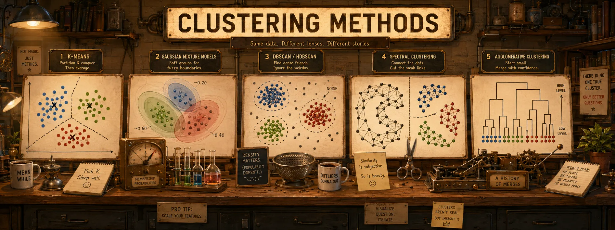
Clustering Methods

Clustering is the part of machine learning where nobody hands the model the answer: you give it points with no labels and it proposes the groups itself. But "what are the groups" has no single right answer: every algorithm quietly assumes something different about what a cluster even is — a ball around a centre, a dense region, a mixture component, a branch of a tree, a piece cut from a similarity graph — and on the very same data those assumptions disagree, sometimes wildly.

This is a tour of the main methods by the shape they assume. K-means and GMM put a centre — and, for GMM, a covariance — on each group. DBSCAN and HDBSCAN look for connected dense regions and call the rest noise. Spectral clustering cuts a similarity graph; agglomerative clustering builds a whole hierarchy you slice where you like. Each section has a small toy where you can watch the method succeed or fail on the geometry it cares about. How these play out on real text — where the representation you choose often matters more than the method — is its own experiment in text clustering. Everything that comes after the fit — labelling clusters, validating them, tuning — is its companion note, clustering in practice.

---

K-means

K-means is the algorithm everyone reaches for first — simple enough to explain on a whiteboard, and often just good enough to survive into production. That makes it a soft default — "need clustering? use K-means" — but the simplicity is deceptive: K-means has substantial limitations, and applying it where it does not fit reliably gives bad results.

The algorithm

The algorithm starts by choosing K initial centroids, then alternates two steps until convergence:

1. Assignment step. Each point is assigned to the nearest centroid (Euclidean distance).
2. Update step. Each centroid is recomputed as the mean of the points assigned to it.

The two steps repeat until the centroids stabilise.

In practice the k-means++ initialisation chooses initial centroids spread out from each other rather than at random; this speeds up convergence and improves quality, and is the default in scikit-learn.

K-means minimises the sum of squared distances from each point to its centroid — the inertia:

inertia = Σᵢ ‖xᵢ − μ_c(i)‖²

where μ_c(i) is the centroid of the cluster to which point xᵢ is assigned. Lloyd's algorithm is a heuristic; it does not guarantee a global minimum but converges to a local one. Running it from several different initialisations and taking the best result is standard practice — set via n_init in scikit-learn (default 'auto': 1 for k-means++ init, 10 for random init).

Where K-means works

• Dense, low-dimensional data. 2D / 3D visualisations are clustered cleanly by K-means; in such spaces Euclidean distance is meaningful and centroids are real "centres" of groups.
• Geometrically convex clusters. K-means assumes clusters are sphere-like regions around a centre; this works for ordinary blobs in moderate dimensions.
• K is known in advance. K-means requires the number of clusters as input. If K is not known, methods like the Elbow rule (inertia as a function of K, looking for an "elbow") or silhouette score on a grid are used to pick it — extra work, but tractable.

Where K-means works poorly

• Naive K-means on high-dimensional sparse data (raw TF-IDF or bag-of-words on tens of thousands of features). The curse of dimensionality kills the meaningfulness of distances; averaging sparse representations turns centroids into diffuse means over many rare dimensions, so distance differences become weak and hard to interpret; the result has no clear structure. (The fix is a text-specific recipe — TF-IDF → SVD → normalise — covered in text clustering.)
• Clusters of different density or non-spherical shape — lines, rings, complex manifolds. K-means partitions space into Voronoi regions of equal shape around centroids, which is wrong for those geometries. The classic example is two concentric rings: K-means draws a straight border between them, which has no meaning.
• Soft boundaries between clusters. K-means gives only hard assignment. A point sitting between two centroids is arbitrarily assigned to one, even if the realistic answer is "half in each".

Variants

• Spherical K-means — explicitly normalises the centroids and optimises a cosine-like assignment on the unit sphere; useful for dense text embeddings where the angle between vectors matters, not their length. A common practical approximation is ordinary K-means on L2-normalised vectors (the identity ‖x − y‖² = 2 − 2 cos(x, y) holds for unit vectors): it often behaves similarly, but it is not mathematically identical, because centroids in standard K-means are not re-normalised after each update.
• Mini-batch K-means — processes data in batches; necessary when the data does not fit in memory or when N is in the millions.
• K-medoids (PAM) — the centroid is a real point from the data, not a computed mean. Robust to outliers and applicable to non-numeric data.

A related — but conceptually distinct — model is Gaussian Mixture Models (GMM), a probabilistic clustering model with soft assignment and clusters of different shape via covariance matrices. K-means is recoverable as the limiting case of GMM with isotropic covariance and hard assignment, but GMM is its own model rather than a variant of K-means.

---

GMM (Gaussian Mixture Models)

K-means draws a hard, straight-edged boundary and assumes every cluster is the same round size. A Gaussian Mixture Model relaxes both assumptions: it models the data as a blend of K Gaussian "bells", each with its own centre and its own covariance — size, stretch, and orientation. Fitting is by Expectation–Maximisation (EM), alternating between "given the current bells, how much does each point belong to each?" (soft responsibilities) and "given those responsibilities, re-estimate each bell".

In return you get three things K-means cannot. A cluster can be long and tilted rather than a round ball, so on anisotropic or unequal-variance data (exactly where K-means slices across the grain) GMM fits the actual shape. Assignment is soft: every point gets a membership probability in each component, so a point on a boundary comes out honestly "60/40" instead of being arbitrarily snapped to one side. And because the whole model is a real probability density, it hands you likelihoods, useful both for novelty detection (low-density points) and for choosing K by BIC or AIC (see clustering in practice).

In principle K-means is the limiting case of a GMM with isotropic, equal-variance covariances and hard assignment, so GMM covers the same geometric intuition — but with more parameters to estimate and more ways to overfit.

The tell is in the ellipses: K-means keeps carving the space around its centroids while GMM rotates with the cluster, and the score jumps from 0.74 to a clean 1.0. That flexibility is also what gets expensive the moment the dimension climbs, which is the whole of the caveats below.

Cost and caveats

• More parameters. A full covariance per component is d(d+1)/2 numbers; in high dimensions this overfits, so covariance_type is usually dropped to "diag" or "tied". (In high dimensions, diagonal covariance is the usual compromise.)
• Still needs K, and EM converges only to a local optimum — several restarts (n_init) are standard.
• Assumes Gaussians. On genuinely non-Gaussian shapes (rings, crescents) it fails the same way K-means does; that is spectral or density territory.

from sklearn.mixture import GaussianMixture

gmm = GaussianMixture(n_components=5, covariance_type="full", n_init=5, random_state=0)
labels = gmm.fit_predict(X)
proba = gmm.predict_proba(X)   # soft responsibilities, (N × 5)

---

HDBSCAN

If K-means is the default for "I know K and I want a hard partition", HDBSCAN is the default for "I do not know K, the cluster shapes may be arbitrary, and the data has noise that should be separated rather than forced into a cluster". The acronym stands for Hierarchical Density-Based Spatial Clustering of Applications with Noise (Campello, Moulavi & Sander, 2013), and it is one of the strongest defaults for those problems in modern practice.

The idea — clusters as connected dense regions

K-means proceeds from a geometric model: a cluster is a sphere-like region around a centroid, and a point belongs to whichever centroid is closest. HDBSCAN proceeds from a different model: a cluster is a connected region of high density, surrounded by regions of lower density. Points in sparse zones are not glued onto the nearest cluster — they receive a separate label -1, meaning "noise".

Two consequences follow. First, clusters can have arbitrary shape — lines, crescents, concentric rings, manifolds — because what matters is density of connectivity, not Euclidean closeness to a centre. Second, the number of clusters is not specified anywhere; it follows from the structure of the data through the min_cluster_size parameter.

The difference from classic DBSCAN is in handling clusters of different densities. DBSCAN uses one fixed neighbourhood radius eps for the whole dataset, which forces a single density threshold; on real data with mixed-density clusters this is too rigid (a small eps tears large clusters apart, a large eps glues everything together). HDBSCAN considers a hierarchy of densities and selects the most stable clusters at appropriate density levels per region of the data — which makes it robust on the kind of mixed-density structure typical of real text and embedding data.

How the algorithm works

Inside HDBSCAN there are four steps. Understanding them helps with parameter tuning.

Mutual reachability distance. For each point, core_k(x) is computed — the distance to its k-th nearest neighbour, where k = min_samples. The pairwise distance is replaced by the mutual reachability:

mrd(a, b) = max(core_k(a), core_k(b), d(a, b))

This metric artificially pushes apart points in sparse regions while leaving dense-region distances unchanged. It is the geometric trick that equalises clusters of different density.

Minimum spanning tree (MST). A minimum spanning tree is built on the mutual-reachability distances. Long edges in the MST correspond to crossings of sparse "intercluster" regions; short edges correspond to dense within-cluster connections.

Hierarchy and condensed tree. From the MST a dendrogram of all possible clusterings at different density thresholds is built and then "condensed": small fluctuations where individual points break off are smoothed into noise. The min_cluster_size parameter sets the threshold below which a branch is considered noise rather than a separate cluster.

Extraction via stability. For each potential cluster, a stability score is computed — how long the cluster persists as the density threshold varies. The most stable branches become final clusters. This is where the automatic choice of K comes from: the data dictates how many clusters their density structure justifies.

Parameters and their effect

HDBSCAN has only a handful of parameters, but each one swings the result hard. Roughly in the order you reach for them:

• min_cluster_size — the main parameter. Minimum size of a group still considered a cluster. Setting it to 3 finds small thematic niches; setting it to 50 finds only large basic topics. Typical values: 20–50 for exploratory survey of large corpora, 5–15 for fine-grained segmentation. The only mandatory parameter.
• min_samples — how many neighbours a point must have to be a "core point". Controls the algorithm's strictness about noise. Small values (1–5) are sensitive to dense regions and assign borderline points to clusters; large values (10–20) increase noise but raise cluster purity. By default equals min_cluster_size; a useful empirical rule is to set it 2–5× smaller.
• cluster_selection_method — 'eom' (excess of mass, the default) selects the most stable clusters and tends to merge related sub-clusters into larger ones; 'leaf' takes the leaves of the dendrogram and gives smaller, more thematically narrow clusters. For exploratory analysis, leaf is often the more useful choice: it is easier to merge fifty narrow topics by hand than to work out what went into ten blurry ones.
• cluster_selection_epsilon — soft merging of close clusters with mutual distance below the specified threshold. Useful when min_cluster_size is correct but the algorithm still fragments related topics.
• metric — the distance used in the mutual-reachability construction. See below for the embedding-specific choice.

Distance on L2-normalised embeddings

For text embedding vectors, what matters semantically is the angle between vectors, not their length — semantic similarity is cosine. HDBSCAN's implementation in the hdbscan library is optimised for Euclidean and is noticeably slower on cosine. The trick from the K-means section applies here too: if all vectors are L2-normalised (which SentenceTransformer and FastEmbed usually do by default for E5-style models), then

‖x − y‖² = 2 − 2 · cos(x, y)

— Euclidean is monotonically equivalent to cosine. Methods that depend only on the order of distances (and HDBSCAN does) should give equivalent neighbour orderings in exact arithmetic, so in practice Euclidean on L2-normalised embeddings is usually the faster way to approximate cosine-based clustering. Edge cases — ties, approximate-neighbour shortcuts in the hdbscan library, finite-precision rounding — can produce small differences in the final partition, but the typical result is effectively the same as cosine.

Noise as a first-class category

HDBSCAN is one of the few common clustering algorithms — the density-based family, DBSCAN included — where "this point does not belong to any cluster" is a normal, expected outcome. Such points get the label -1 and should not be ignored when analysing results.

The share of noise is itself a useful diagnostic. In many exploratory text-clustering workflows 5–20% noise is a healthy range — there are always idiosyncratic points that do not fit into large groups — though other corpora legitimately run higher or lower. Above 50% usually means min_cluster_size is too large for the available data; near 0% means it is too small and clusters are absorbing everything indiscriminately. The noise fraction works as a cheap signal for calibrating min_cluster_size.

The contrast with K-means is qualitative. K-means must assign every point somewhere, so isolated outliers get dragged into the nearest centroid and pollute its cluster. HDBSCAN sets them aside, which is at once more honest and more practical: noise can be reviewed separately (manually inspected, sent for re-labelling, or simply left alone) without contaminating the interpretation of the other clusters.

When to use HDBSCAN

The setting where HDBSCAN is the strongest default is semantic grouping of short user messages with an unknown number of topics and a noticeable fraction of irregular requests — chat logs, search queries, reviews, support tickets. The cluster-size distribution in such corpora is sharply uneven (a few massive top topics plus a long tail of niches) and the noise share is a real artefact that deserves explicit handling. Other density-based methods exist (OPTICS, mean-shift), but HDBSCAN's combination of automatic K selection, mixed-density tolerance, and explicit noise label is what makes it the typical pick.

Compared to Agglomerative, HDBSCAN avoids the K-equivalent threshold-choice problem and the quadratic memory complexity. Compared to K-means, it does not require knowing K, does not assume spherical clusters, and honestly separates noise.

On real text, HDBSCAN is usually the last step of an embeddings → UMAP → HDBSCAN pipeline — the BERTopic recipe — and that side of it lives in text clustering.

Its home turf is well-separated groups of uneven density sitting in a field of noise, with the number of groups unknown. There the one thing K-means structurally cannot do — decline to assign a point — is exactly what the data needs.

Flip between the two and the difference is not subtle. K-means has to colour the entire background, so the scattered noise quietly poisons all three clusters; HDBSCAN just greys it out and keeps them clean. That single ability, to say a point belongs to nothing, is most of what you are paying for.

---

DBSCAN

I put HDBSCAN first because it is the version I reach for in practice — but it is the refinement of an older, simpler idea worth understanding next: DBSCAN (Density-Based Spatial Clustering of Applications with Noise, 1996). DBSCAN defines a cluster as a chain of points each with enough neighbours within a fixed radius, and labels everything else noise. No K, arbitrary shapes, explicit outliers — the same headline strengths as HDBSCAN.

The two parameters

• eps — the neighbourhood radius. A point is a core point if at least min_samples points lie within eps of it; clusters grow by connecting core points whose neighbourhoods overlap.
• min_samples — how many neighbours make a point "core". Higher values demand denser regions and produce more noise.

The single-eps problem — and why HDBSCAN exists

DBSCAN's weakness is that eps is one global radius for the whole dataset. When clusters have different densities, no single eps fits all of them: set it small and the sparse clusters shatter into noise; set it large and the dense clusters merge. There is often no value that gets both right.

HDBSCAN's contribution is exactly this: instead of one eps, it considers a hierarchy of density thresholds and keeps the most stable clusters at whatever density each region of the data calls for. On a single, uniform density DBSCAN is simpler and perfectly good; the moment densities vary, reach for HDBSCAN.

from sklearn.cluster import DBSCAN

db = DBSCAN(eps=0.5, min_samples=10).fit(X)
labels = db.labels_   # -1 marks noise

Picking eps is usually done with a k-distance plot: sort every point's distance to its min_samples-th neighbour and look for the "knee" — the distance at which the curve bends sharply upward.

---

Spectral clustering

K-means asks "which centroid is each point nearest to?" and HDBSCAN asks "which points share a dense region?". Spectral clustering asks something different: treat the data as a graph and cut it where the connections are weakest. That lets it recover clusters none of the centroid- or density-based methods can — shapes that curve, interlock, or wrap around one another.

The idea — cluster the graph, not the points

Three steps:

1. Build a similarity graph. Connect each point to its near neighbours (k-nearest-neighbours, or a Gaussian/RBF kernel on the distances). The result is an affinity matrix with high weights between similar points and ~0 between distant ones.
2. Embed via the graph Laplacian. Form the Laplacian L = D − A (with A the affinity and D its degree matrix), take its smallest few eigenvectors, and use them as new coordinates. This spectral embedding unfolds the graph so that points well-connected through it land close together — even when they sit far apart in the original space.
3. Cluster the embedding. Run ordinary K-means on those few eigenvector coordinates. The embedding has already done the geometric work, so a simple straight-edged partition there corresponds to a complex, curved partition back in the original space.

Two concentric rings are separable by no straight line, but in the graph they are two essentially disconnected components — so in the spectral embedding they collapse to two tight, far-apart blobs that K-means then splits trivially.

This is the one demo where K-means does not merely score worse, it scores nothing: ARI around zero on the rings, because no straight line will ever separate them. Spectral gets a perfect 1.0. It is the cleanest right-tool / wrong-tool split in the whole note.

Where it works

• Non-convex, interlocking shapes — rings, moons, spirals, manifolds. This is the signature strength and the reason to reach for it: precisely the geometries where K-means draws a meaningless straight border.
• Small-to-medium datasets where a good affinity graph can be built and the eigendecomposition is affordable.
• When a meaningful similarity exists even if Euclidean distance does not — any affinity (graph, kernel, learned) plugs in.

Where it struggles

• Cost. The eigendecomposition of an N×N Laplacian is roughly O(N³) in the dense case — cheaper with sparse kNN graphs and approximate eigensolvers, but still the binding constraint. Spectral clustering does not scale to millions of points the way mini-batch K-means or indexed HDBSCAN do.
• K is required, exactly as for K-means — it is the number of eigenvectors, and of final clusters.
• Sensitivity to the affinity. The whole result rides on how the graph is built — the neighbour count, or the kernel bandwidth. A badly scaled affinity gives a badly behaved embedding; this is the main tuning lever and the main failure mode.

Using it in practice

from sklearn.cluster import SpectralClustering

sc = SpectralClustering(n_clusters=2, affinity="nearest_neighbors",
                        n_neighbors=10, assign_labels="kmeans", random_state=0)
labels = sc.fit_predict(X)

affinity="nearest_neighbors" builds a sparse kNN graph — robust, and the usual default for shape-finding; affinity="rbf" uses a Gaussian kernel whose gamma bandwidth is powerful but finicky. On text embeddings spectral clustering is occasionally used as the final step in place of K-means when the geometry is suspected to be non-convex — but on the roughly-convex blobs that good embeddings tend to produce, plain K-means is usually just as good and far cheaper.

---

Agglomerative (hierarchical) clustering

Every method so far hands you a flat partition at one chosen K. Agglomerative clustering hands you the whole hierarchy: start with every point as its own cluster, repeatedly merge the two closest clusters, and record the order. The result is a dendrogram — a tree of merges — and you read clusters off it by cutting at a height of your choice.

Linkage — what "closest" means

The merge rule (the linkage) shapes the result:

• ward — merge the pair that least increases within-cluster variance. Euclidean only; the usual best default for compact, roughly-spherical clusters.
• average — mean pairwise distance between clusters; robust, works with any metric.
• complete — maximum pairwise distance; gives tight, equal-diameter clusters.
• single — minimum pairwise distance; can follow elongated shapes, but is prone to "chaining" stray points together, so it is usually avoided.

The nice part is that you do not have to commit to K before fitting; you inspect the tree and choose a cut afterwards. The big vertical jump between the three-cluster and six-cluster heights is the data telling you which scales are real and which are arbitrary.

When to use it

• You don't know K and want to see structure at every level. The dendrogram shows the whole nesting at once — cut high for a few broad groups, low for many fine ones, all from one fit.
• Small-to-medium datasets. The catch is cost: building the full tree is O(N²) memory and worse in time, which rules it out much above ~30k points (a 50k×50k distance matrix is already ~10 GB). For larger data the flat methods above scale far better.
• No K is required — a distance threshold replaces it — and the dendrogram is itself a useful artefact for communicating structure to people.

from sklearn.cluster import AgglomerativeClustering

agg = AgglomerativeClustering(n_clusters=5, linkage="ward")   # or distance_threshold=...
labels = agg.fit_predict(X)

---

Comparative table of clustering methods

The table below isn't a ranking — no method wins outright. Each one solves a problem by handing you another: K-means asks you for K, HDBSCAN asks you what counts as a real cluster, DBSCAN asks you for one global density, spectral clustering asks you to pay for the graph, and NMF asks whether topics are enough instead of clusters. (It also lists a few close cousins — LDA, mini-batch and spherical K-means, BERTopic — that don't get their own section above.)

Method	Input	Requires K	Soft assignment	Complexity	Interpretation	When to use
K-means	Dense vectors	yes	no (hard)	O(N·K·d·iter)	centroid	Dense + known K
Mini-batch K-means	Dense vectors	yes	no (hard)	O(B·K·d·iter)	centroid	Very large N (>1M)
Spherical K-means	L2-normalised vectors	yes	no (hard)	O(N·K·d·iter)	centroid	Embeddings + known K
NMF	Sparse TF-IDF	yes	yes (soft)	O(N·K·V·iter)	topic-word	Topic modelling
LDA	Bag-of-words	yes	yes (probabilistic)	slower than NMF	topic-word	Probabilistic topic modelling
GMM	Dense vectors	yes	yes (probabilistic)	O(N·K·d²·iter)	mean + covariance	Soft, elliptical clusters
Agglomerative	Vector + metric	no, but needs a cut	no (hard)	O(N²) memory, O(N² log N) time	dendrogram	Small datasets (≤30 k)
DBSCAN	Vector + metric	no	no + outliers	O(N²) naive, O(N·log N) with kNN index	density-based	Arbitrary shapes, known density
HDBSCAN	Vector + metric	no	no + outliers	O(N²) naive, O(N·log N) with kNN index	exemplars	Dense + unknown K + noise
Spectral	Vector + affinity	yes	no (hard)	O(N²) graph, O(N³) eigendecomp	graph cut	Non-convex shapes, small N
BERTopic	Text	no	no (hard)	dominated by HDBSCAN + UMAP	c-TF-IDF	Modern text topic-modelling pipeline

The near-O(N log N) for DBSCAN and HDBSCAN assumes a low-dimensional, indexable space; on high-dimensional embeddings the neighbour index degrades and the cost drifts back toward O(N²).

Practical bounds by size

These are not hard thresholds but levels at which problems with memory or time usually start.

• Up to 10 000 points. Practically everything works, including Agglomerative. Choose by other criteria.
• 10 000 – 100 000. Agglomerative starts running into memory limits (a 50 k × 50 k pairwise-distance matrix in float32 is ~10 GB). For embeddings, HDBSCAN or K-means; for TF-IDF, the standard SVD-based pipeline.
• 100 000 – 1 000 000. HDBSCAN with an index and K-means remain operable, but the time/quality ratio becomes noticeable. UMAP-based preprocessing can help, with the usual caveat: cluster on the full embeddings, not on the 2-D UMAP output.
• Above 1 M. Mini-batch K-means or distributed solutions (Spark MLlib KMeans, FAISS-based pipelines). HDBSCAN is usually run on a sample, then the remaining points are assigned to the nearest discovered clusters via kNN / approximate nearest neighbours.

---

There is no generic best clustering algorithm. Each one is a bet on what shape the groups in your data have — a centre, a covariance, a density basin, a graph cut, a branch of a tree. Get the shape right and the method nearly picks itself; get it wrong and no amount of tuning rescues it. Which shape your text actually has — and why the representation often decides more than the method — is the experiment in text clustering.