Chapter 14 of 14
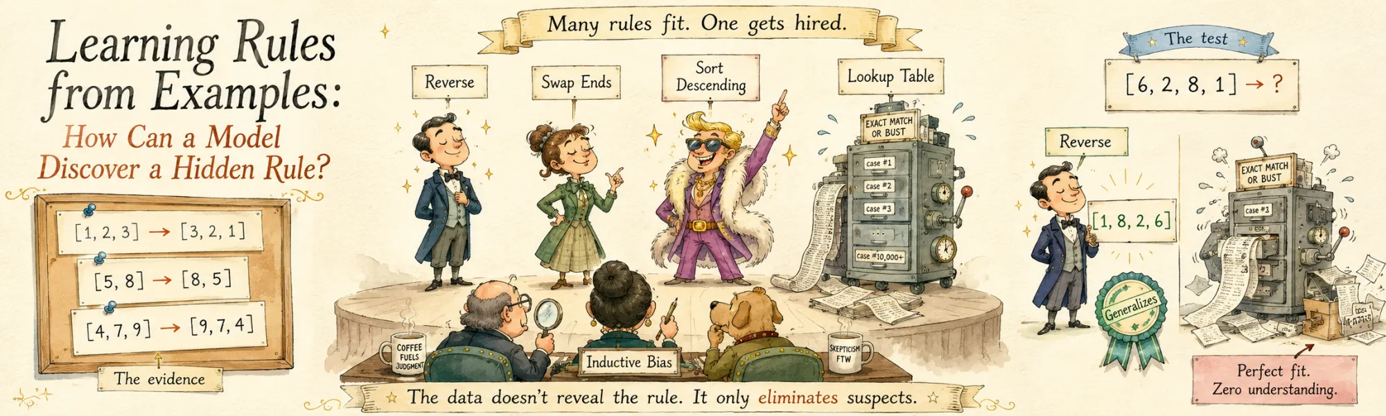
Learning Rules from Examples: How Can a Model Discover a Hidden Rule?
Created Aug 9, 2026
Most machine learning problems are presented in one direction: we have data, we train a model, we ask it to predict something new. But there is a simpler version of the same problem, and it exposes something surprisingly deep. Suppose I show you this:
[1, 2, 3] → [3, 2, 1]
[5, 8]    → [8, 5]
[4, 7, 9] → [9, 7, 4]
What should happen to [6, 2, 8, 1]? Almost everyone answers [1, 8, 2, 6] within a second: the hidden function reverses the sequence. But something strange has already happened. Nobody told you the rule — you inferred it from three examples — and reverse is not the only rule that fits. Infinitely many functions produce exactly those three outputs, including this one:
def mysterious_function(x):
    if x == [1, 2, 3]:
        return [3, 2, 1]
    if x == [5, 8]:
        return [8, 5]
    if x == [4, 7, 9]:
        return [9, 7, 4]
This ridiculous function fits the evidence perfectly, and nobody would seriously propose it. Why not? That single question opens onto a large part of machine learning: induction, hypothesis spaces, inductive bias, identifiability, generalization, active learning, compositionality, and the problem of telling genuine structure apart from shortcuts that merely correlate with it.
I worked through those ideas by building a tiny artificial world where the rules are hidden and I control exactly what the learner is allowed to see, and then running nine experiments in it — on three local open-weight models (Qwen3 at 8B, 30B-A3B and 32B, 4-bit, on a laptop) and on two tiers of a frontier model. The goal was never a useful production system. The goal was to make learning visible: small enough that when a learner gets the rule wrong, we know precisely which rule it should have found, how many bits of evidence it had, and which of several distinct failures actually occurred.
Three of the results cut against the usual intuition. The most capable model in the study is the one most easily fooled by a correlated feature. The weakest model, whose proposed rules usually contradict the very examples it was shown, still supplies as much useful search guidance as a hand-written heuristic. And the classic argument that program search dies of combinatorial explosion is wrong in this setting by two orders of magnitude — measured, not argued.
Runnable companion. The Learning Rules from Examples lab holds the code for every experiment below — the language, the task generator, the version space, the verifier and each of the nine experiments — written out in full and ready to run. It builds the world step by step instead of reporting it, and the experiments run against whatever models you point it at — local weights, an API, or a mix.
The setting has an obvious full-scale relative: ARC (Chollet, On the Measure of Intelligence, 2019), a benchmark of grid puzzles built on exactly this premise — a handful of demonstrations, one hidden transformation, no task-specific training process. The difference is deliberate. ARC is hard partly because nobody knows what its hypothesis space is; here the hypothesis space is a thing I write down, shrink, corrupt, and enumerate. That control is the entire point, and it is what lets every claim below be settled by a deterministic verifier rather than by a benchmark number.
From rules to examples, and back again
Give me a rule — reverse the sequence — and an input [3, 8, 1], and the problem is trivial: apply the rule to the data. That direction is deduction, rule + input → output. The original puzzle runs backward, input/output examples → unknown rule: we observe what a system does and try to infer the mechanism behind it. That is induction, and in machine learning we do it constantly, only with a hidden function far less interpretable than reverse. Given examples we want a function with that also works on inputs we have never seen.
That last clause carries nearly all the weight. Fitting the observations is easy — the lookup table above does it in four lines. Finding something that generalizes is the hard part, and it is not a matter of trying harder at the fitting. It is a question about what happens off the data, where the data by construction says nothing.
Formal learning theory has a name for the version of this question that asks whether the data can ever pin the rule down. Gold's identification in the limit (1967) asks whether a learner fed an infinite stream of examples eventually settles on the correct hypothesis and never changes its mind again. The answer depends entirely on the class of rules under consideration, not on the learner's cleverness — some classes are identifiable from positive examples alone, others provably are not. That framing is the right one to keep in mind here: every question below is really a question about the pair (hypothesis class, evidence), never about the learner alone.
Many rules fit the same evidence
Take a single observation, [1, 2, 3] → [3, 2, 1]. The rule could be reverse. It could equally be swap first and last, or sort descending, or some special-cased rotation for length-three inputs, or an arbitrary lookup table. With one observation the hidden function is hopelessly underdetermined. Add [4, 9] → [9, 4] and some explanations get less attractive, but reverse and swap_first_last remain perfectly indistinguishable — on length-two inputs they are the same function. Only a third example with a moving middle, [7, 2, 5, 8] → [8, 5, 2, 7], separates them.
This is the first load-bearing idea: a dataset does not specify a rule, it eliminates hypotheses. Learning is then maintaining — explicitly or implicitly — the set of explanations still standing, and watching that set shrink as evidence arrives. Stated that way it is not a new idea at all: it is Mitchell's version space (Generalization as Search, 1982), the set of all hypotheses in a fixed language consistent with the data so far, and the candidate-elimination algorithm that maintains it. With a small enough language we can be completely literal about it:
consistent = [h for h in HYPOTHESES if all(h(x) == y for x, y in examples)]That is a complete learner. It is also a measuring instrument, which is what I actually want it for, because it turns a vague statement — "the space narrows" — into a number. If the language is finite and we hold a uniform belief over the survivors, the uncertainty about the rule after examples is exactly
and each new example is worth precisely the number of bits it removes. An example that eliminates nothing is worth zero bits, no matter how much it looks like data. This is the quantity I will keep coming back to, and it is the reason the toy world earns its keep: in a real problem you cannot count the surviving hypotheses, and here you can.
Stating it in bits also buys a free lower bound. Identifying one hypothesis out of requires bits to arrive from somewhere, and a single demonstration can carry at most the log of the number of outputs it could possibly have taken. Divide the one by the other and you have a floor on the number of demonstrations that no learner — neural, symbolic, or human — can go below. Much of what looks like a model failing to induct is a model being handed fewer bits than the answer costs, and in this world we can tell the two apart by construction.
One warning about this learner before it does any work. Elimination is brittle in exactly one way: a single mislabeled example deletes the true hypothesis permanently, and the learner then confidently converges on something else, or on nothing at all. The repair is to stop treating consistency as a hard constraint and score hypotheses by how many examples they get wrong. With an independent error rate per demonstration, a hypothesis that misses of examples has likelihood
so the posterior ranks hypotheses by error count, and hard elimination is the limit in which any single error is fatal. That formula is worth keeping in view, because the next section leans hard on the opposite case — and this is exactly where its argument stops applying. Everything below assumes noiseless demonstrations unless stated otherwise; the noisy variant is a knob in the task generator, and it changes which learner is even admissible.
A tiny hypothesis space
To make any of this concrete I need a language of transformations. Everything in it maps list[int] → list[int] — one type in, one type out — which is not a cosmetic decision: it makes every composition well-formed, so a program is just a chain and search never has to reason about types. The primitives:
def identity(x):       return x
def reverse(x):        return x[::-1]
def rotate_left(x):    return x[1:] + x[:1]
def rotate_right(x):   return x[-1:] + x[:-1]
def duplicate(x):      return x + x
def every_second(x):   return x[::2]          # 0-based: keeps positions 0, 2, 4, ...
def increment(x):      return [v + 1 for v in x]
def double(x):         return [2 * v for v in x]
def swap_ends(x):      return [x[-1]] + x[1:-1] + [x[0]] if len(x) > 1 else x
def sort_asc(x):       return sorted(x)
def sort_desc(x):      return sorted(x, reverse=True)
def keep_last(x):      return x[-1:]
def keep_max(x):       return [max(x)] if x else []
def decrement(x):      return [v - 1 for v in x]
def pairwise_swap(x):  return [v for a, b in zip(x[::2], x[1::2]) for v in (b, a)] + (x[-1:] if len(x) % 2 else [])
Two of those names deserve a note, because both encode a decision that bites later. every_second keeps positions 0, 2, 4 — Python's x[::2], and if you call the same operation "drop the even positions" you will be reading a 1-based description of 0-based behaviour and will eventually mis-grade a model that got it right. And selectors like keep_last return a one-element list, not a scalar. That keeps the type discipline intact, and it is what lets the shortcut experiment below live in the same DSL as everything else instead of quietly becoming a different problem.
Now the game: pick a hidden function, generate examples from it, ask a learner to recover it. At depth one this is almost embarrassingly simple — which is exactly what makes it useful, because anything interesting that happens has a knowable cause.
Experiment 1 — recovering a hidden operator
The hidden function is rotate_left, but the learner never sees the name. It sees only
φ([1, 2, 3, 4]) → [2, 3, 4, 1]
φ([8, 5, 9])    → [5, 9, 8]
φ([7, 6])       → [6, 7]
and is asked for φ([a, b, c, d, e]). There are three genuinely different things we can ask it to produce: the output ([b, c, d, e, a]), a description of the rule ("move the first element to the end"), or an executable program (lambda x: x[1:] + x[:1]). These look interchangeable and are not. A system can predict several test outputs correctly without ever representing the rule in reusable form, and it can describe the rule perfectly while botching execution on a long input.
That splits "did it learn the rule?" into four quantities, and they have to be measured separately or the interesting part disappears. Rule identification — but graded by compiling the stated rule and checking it is extensionally equal to the hidden function on a fixed probe set, never by string-matching English. "Move the last element to the front, no wait, the first to the end" is correct if it compiles to the right behaviour. Output prediction — is the transformed list right. Self-consistency — does the learner's own program reproduce the demonstrations it was just shown; note that this one is checkable without knowing the answer. And whether the reply parsed at all.
Fourteen primitives, fifteen seeds each, three demonstrations per task, the primitive menu in the prompt. Before grading, every task is checked against all 115 behaviours reachable at depth ≤2: 65 of 70 are pinned uniquely by their demonstrations, so a failure here is the learner's, not the evidence's.
| learner | rule | output | self-consistent | consistent-but-wrong |
|---|---|---|---|---|
gpt-5.6-luna | 1.00 | 1.00 | 1.00 | 0 |
| Qwen3-32B | 0.638 ±0.065 | 0.657 | 0.643 | 1 |
| Qwen3-30B-A3B | 0.543 ±0.067 | 0.533 | 0.543 | 0 |
| Qwen3-8B | 0.367 ±0.065 | 0.443 | 0.371 | 1 |
The frontier model is perfect on all fourteen primitives, so the interesting content is entirely in the local gradient — and in the last column.
Across 630 local calls there are exactly two plausible-but-wrong hypotheses. Every other failure — 24, 32 and 43 of them — proposes a program that does not reproduce the three demonstrations the model had just read. On one task where the evidence left 0.00 bits of ambiguity, Qwen3-8B answered rotate_left → swap_ends, which breaks on the very first demonstration. These are not competing explanations of the data; they are answers that never fit it.
That has a consequence worth stating plainly, because it is the strongest practical result in the note: the failures of weak models here are caught by a two-line check that never sees the ground truth. Run the proposed program on the demonstrations. If it disagrees, discard it. No oracle, no labels, no benchmark.
Two smaller findings fall out. Predicting the output is easier than naming the rule on the weak models (8B: 0.443 against 0.367), which is the Task A / Task B split showing up as a gap rather than an argument. And the difficulty is entirely structural: elementwise arithmetic — double, increment, duplicate — is 5/5 for every model including the 8B, while everything positional — swap_ends, pairwise_swap, every_second, rotate_right — sits at 0–2/5 on locals and 5/5 on the frontier.
Removing semantic hints
There is an obvious problem with building an induction study on reverse. A language model has seen sequence reversal an enormous number of times; renaming it flibble hides the label, not the concept. Whatever such a task measures, it is contaminated by recall, and for the LLM learners below that contamination is not hypothetical — these are exactly the transformations that appear in every tutorial in the training corpus.
The fix is to make the rule local to the experiment: sample it at runtime. Draw a permutation
permutation = [2, 0, 3, 1] # position i of the output takes input element permutation[i]and define . The operator's name carries no information, and with a fresh permutation per run the exact mapping did not exist as a named task before the run started. There are of them for arity — 24 at length 4, 5040 at length 7 — which is small enough to enumerate exhaustively and large enough that nothing is memorized.
One property of has to be stated rather than discovered later: a permutation operator is defined for exactly one input length. has nothing to say about a five-element list. So the permutation world is a fixed-arity world — all demonstrations and all tests share length — and it is the right instrument for questions about evidence and identifiability, where I want a hypothesis space I can count. It is the wrong instrument for questions about length, and the length-generalization experiment below therefore uses only length-polymorphic primitives from the DSL. Mixing the two would produce a beautiful graph measuring nothing.
This is the general case for synthetic environments, and it is not realism — it is control. Here we know the true rule, exactly which information was shown and which withheld, which alternative hypotheses exist and how many, and whether a test input is genuinely novel. On a natural-language benchmark, not one of those five is guaranteed.
Experiment 2 — how much evidence is enough?
Hidden operator: for a freshly sampled permutation of arity 5, so the hypothesis space is all permutations — bits to spend. Demonstrations arrive one at a time, , in two conditions that differ only in the alphabet the inputs are drawn from: values , where positions collide, and values , where they rarely do. Twelve seeds per cell, and after every example the exact version space is recomputed, so each task carries its own floor.
The floor alone already answers half the question, before any model is involved:
| condition | |||||
|---|---|---|---|---|---|
| values — bits remaining | 2.71 | 1.00 | 0.33 | 0.00 | 0.00 |
| — identified | 0/12 | 1/12 | 8/12 | 12/12 | 12/12 |
| values — bits remaining | 1.26 | 0.08 | 0.00 | 0.00 | 0.00 |
| — identified | 2/12 | 11/12 | 12/12 | 12/12 | 12/12 |
The alphabet, not the number of examples, is what makes this task hard. With distinct values a single demonstration nearly pins the operator; with ties it takes five. Same rule, same learner, same count of examples — different amount of information, exactly as the teaching-dimension argument below predicts.
Now the learner. gpt-5.6-luna, on the same 120 tasks:
| tasks | named the right permutation | named a permutation consistent with every demonstration | |
|---|---|---|---|
| evidence sufficient (0 bits) | 82 | 0.976 | 1.000 |
| evidence insufficient (>0 bits) | 38 | 0.368 | 1.000 |
That second row is the result. 0.368 is not an error rate — it is approximately the chance of guessing right among the survivors. In every one of the 38 under-determined tasks the model named a permutation that reproduces all the evidence it was given. It did the only thing that can be done, and the residue is the ambiguity, not the model.
Escalating to the more expensive gpt-5.6-terra on the identical tasks changes nothing: 0.988 when the evidence suffices, against luna's 0.976. Where a task is decided, both tiers decide it; where it is not, no tier can.
The two remaining failures at maximum evidence are worth quoting, because they are not inference failures at all:
truth [0, 2, 4, 3, 1]   named [0, 2, 3, 4, 1]
truth [4, 0, 3, 1, 2]   named [4, 0, 1, 3, 2]
Both are a single adjacent transposition, both at positions 2–3, both with ten demonstrations in view and zero bits of ambiguity. They look far more like transcription slips than failures to identify the permutation — though the output alone cannot settle which it was. That is the identification-versus-execution split of a later section, appearing here uninvited.
And the more interesting record is not the accuracy at all. It is which wrong rule the learner names when the evidence is insufficient — because with the true hypothesis not yet identified, whatever it picks is a direct readout of its prior. That is the next section's subject, and Experiment 2 has already collected the data for it.
Inductive bias: why some rules feel better
Back to the opening question. Two hypotheses explain [1,2,3] → [3,2,1] and [4,5] → [5,4]: reverse and the four-line lookup table. Why is one obviously right?
Here the toy setting pays off, because it admits a sharp answer rather than an appeal to taste. Both hypotheses are deterministic, so the likelihood of the observed data is binary: if reproduces every example, otherwise. Bayes then gives
The data does exactly one thing: it deletes the inconsistent hypotheses. Among the survivors, the entire choice is made by the prior — the likelihood has no opinion left to offer. Inductive bias is not a thumb on the scale in this setting; it is the whole scale. That is why the phrase "let the data speak for itself" is incoherent for problems shaped like this one, and why two learners with identical training performance can disagree about everything off-distribution. (Note where this stops: put the noise term from the previous section back in and the likelihood recovers its voice, ranking survivors by error count. The claim that the prior decides everything is exactly a claim about noiseless data.)
The strongest version of the point is older and does not need Bayes at all. Watanabe's ugly duckling theorem shows that if you refuse to privilege some predicates over others, then any two objects share exactly as many properties as any other two — every pair is equally similar, so no generalization is possible even in principle. A learner with no bias is not a cautious learner; it is not a learner.
The classic prior is a description-length one, for the length of in some coding scheme — Solomonoff's induction in idealized form, MDL in practice, and the reason it is not merely aesthetic is Occam-style learning theory (Blumer et al., 1987): a learner that compresses its data generalizes, with a sample-complexity bound in terms of the compression. Apply it to the two candidates. reverse has a length that does not depend on how many examples it explains. The lookup table has to name every case, so grows linearly in , and the posterior odds against it fall off like — after five examples the "rule" that memorizes them is exponentially worse-supported than the rule that generates them, even though both fit the data exactly. That is the formal content of the intuition, and it is why nobody proposes mysterious_function while everyone proposes reverse.
Where does a real learner's bias come from? For humans, some mix of preferences for simplicity, uniformity, and reusability. For a neural model, it is distributed across architecture, training distribution, regularization, representation, and search procedure, and it is not something we get to read off directly — which is why Experiment 2 records the wrong answers. For an in-context learner specifically there is a useful theoretical story: in-context learning behaves like implicit Bayesian inference over latent tasks, with the pretraining distribution supplying the prior (Xie et al., 2021), and the mechanism that makes pattern continuation possible at all is at least partly identifiable in the weights as induction heads (Olsson et al., 2022) — the "find the previous occurrence and copy what followed" circuit that the mechanistic interpretability note reproduces and ablates. That is the honest reason to run these experiments on a language model rather than only on a symbolic learner: the prior is not designed, it is inherited, and the only way to find out what it contains is to probe it.
The prior, measured
Experiment 2 left 38 tasks where the evidence genuinely did not decide, and in every one of them gpt-5.6-luna named a permutation consistent with all the data. So the question "which survivor does it prefer?" is well posed, and answerable.
Take displacement — the number of positions a permutation moves relative to identity — as a simplicity proxy. The baseline is computable exactly rather than guessed: a uniform random pick from the version space lands on a least-displaced survivor 51.2% of the time, with mean displacement 4.05.
| learner | answers inside the version space | picks a least-displaced survivor | exact two-sided |
|---|---|---|---|
gpt-5.6-luna | 38/38 | 28/38 = 0.74 | 0.006 |
gpt-5.6-terra | 36/37 | 26/36 = 0.72 | 0.012 |
| Qwen3-32B | 19/38 | 12/19 = 0.63 | 0.36 |
| Qwen3-8B | 12/38 | 9/12 = 0.75 | 0.15 |
| Qwen3-30B-A3B | 25/38 | 12/25 = 0.48 | 0.84 |
The frontier models carry a real simplicity bias — 23 points above chance, mean displacement 3.68 against the version space's 4.05 — and the preference did not strengthen between these two tiers. Two points is not a trend, but it is at least evidence that this is not simply bought with more compute.
The local models are the more instructive row, because for them the question cannot be asked. Only 12 to 25 of their 38 answers land inside the version space at all; on subsamples that small every estimate overlaps chance. You cannot measure a learner's prior over the surviving hypotheses unless the learner is choosing among them, and a learner whose answer contradicts the demonstrations it was shown is not choosing among them — it is somewhere else entirely. Hold onto that: it decides what such a model is good for, and the search section will cash it in.
So the question is never "which hypothesis fits the data" — that set is computable and usually large. It is which of the fitting hypotheses the learner prefers, and that is an empirical property of the learner.
Experiment 3 — an ambiguous dataset, built on purpose
Let the true rule be keep_last. Now construct demonstrations in which the last element also happens to be the maximum:
[1, 3, 7]  → [7]
[2, 4, 9]  → [9]
[3, 8, 10] → [10]
Two hypotheses in the DSL explain every example: keep_last and keep_max. On the training evidence they are indistinguishable — not approximately, exactly. Then the disambiguating test, [9, 2, 4], where the true rule predicts [4] and the shortcut predicts [9].
This is a miniature of one of the largest failure modes in deployed machine learning: perfect training performance on a feature that merely correlates with the intended rule, invisible until the correlation breaks (Geirhos et al., Shortcut Learning in Deep Neural Networks, 2020 — the Clever Hans story with gradients). The toy version shows the entire structure with three rows instead of a million, and it makes the intervention testable: what has to change for the learner to stop taking the shortcut?
Four conditions, 20 seeds. Answer directly; state the rule first, then answer; list every consistent rule first, then commit; or answer, receive one counterexample, and try again. Plus a control in which the demonstrations are descending, so the last element is the minimum and the bait points the other way.
Start with the direct condition, where the ordering across models inverts:
| learner | answers [4] (true rule) | answers [9] (shortcut) |
|---|---|---|
| Qwen3-8B | 0.80 | 0.15 |
| Qwen3-30B-A3B | 0.60 | 0.35 |
| Qwen3-32B | 0.20 | 0.70 |
gpt-5.6-luna | 0.20 | 0.80 |
Across these four learners, susceptibility to the shortcut tracked task performance. The model that was perfect on Experiment 1, that tracks the information floor in Experiment 2, and that designs optimal experiments in Experiment 4, is the one that walks into the trap four times out of five. The weakest model in the study resists it best.
One explanation fits everything else in the note, though the experiment does not establish it: the bait may work because the learner has a strong prior over compact, nameable rules, and keep_max is a far more nameable rule than "the last one, which happens to also be the largest". That is a hypothesis, not a measurement — the prior I did measure was over permutations, a different space — but if it holds, then the property that makes a model good at induction is the same one that makes it exploitable by a correlated feature. Worth stating as a conjecture the design could test, not as something these four models proved.
Now the interventions, and here the ordering reverses:
| learner | direct | rule first | all hypotheses first | candidates it actually listed |
|---|---|---|---|---|
gpt-5.6-luna | 0.20 | 0.15 | 0.80 | 4.8 |
| Qwen3-8B | 0.80 | 0.60 | 0.65 | 1.6 |
| Qwen3-30B-A3B | 0.60 | 0.00 | 0.25 | 2.5 |
| Qwen3-32B | 0.20 | 0.00 | 0.10 | 1.1 |
Two things happen at once, and they point in opposite directions.
Asking for the rule before the answer hurts every learner — 30B falls from 0.60 to 0.00, 32B from 0.20 to 0.00. Naming a single hypothesis is an act of commitment, and the hypothesis that gets named is the seductive one. This runs directly against the reflex to make a model "state its reasoning first."
Asking for every consistent rule rescues the frontier model and nobody else — luna goes from 0.20 to 0.80. The mediator is in the last column: luna genuinely enumerates about five candidates, while the local models produce one or two. And that is exactly what the previous section predicted. Enumerating the version space is only possible for a learner that is in it, and Experiment 2 measured how often each learner's answer contradicts the very demonstrations it was shown. "Consider the alternatives before you commit" is not general advice; it is advice that presupposes the alternatives are visible.
The control settles what the bait actually is. When the demonstrations are descending and the last element is the minimum, the models answer the minimum (luna 0.25, Qwen3-30B 0.45). It is not a preference for maxima. It is a preference for a salient aggregate over a position — the same bias, mirrored. One counterexample repairs luna (0.90) and the 8B (0.85), only half-repairs the 32B (0.55), and does not repair the 30B at all.
Evidence is not just quantity
Suppose the surviving hypotheses are reverse and swap_ends, and I feed the learner [a, b]. Both return [b, a]. That example carries zero bits; ten more length-two examples carry zero bits each. One length-four example, [a, b, c, d], splits them cleanly — [d, c, b, a] versus [d, b, c, a]. Evidence is not a quantity you accumulate, it is a question you ask, and most questions are bad.
With the hypothesis set enumerable, "informative" stops being a metaphor. A candidate query partitions the surviving set into groups by the output each hypothesis predicts, . Since the hypotheses are deterministic, observing eliminates everything outside , so under a uniform posterior the expected information gain of the query is exactly the entropy of that partition:
The best query is the one that splits the survivors most evenly; a query on which every hypothesis agrees has ; the ceiling is , attained when the query separates every hypothesis from every other. This is computable by brute force in our world, which gives us something to grade a model against — but it is worth being precise about what. Maximising one-step gain is generalized binary search, and greedy is not the optimal querying policy: Dasgupta (2004) bounds greedy GBS within a factor of the optimal decision tree, and Golovin & Krause's adaptive submodularity gives the -style guarantee for version-space reduction. So what the experiment below reports is regret against a greedy oracle, which is a slightly weaker yardstick than it first sounds.
The shift in framing is the point. Instead of what can I infer from the examples I was given, the learner asks which example should I request next — active learning, and a different kind of competence.
The teaching dimension
There is a third quantity hiding here, and naming it turns the whole section from an intuition into arithmetic. Ask not what a learner can infer from random examples, and not which example a learner should request, but: what is the smallest set of examples that would pin the rule, if someone who already knew the answer got to choose them? That is Goldman & Kearns' teaching dimension, and for the permutation family of the previous section it has an exact closed form:
for arity over an alphabet of distinct values. The reason is worth seeing, because it is the whole idea of the section in one image. To recover a permutation you must be able to tell the input positions apart, and each demonstration labels every position with one symbol from the alphabet. So a teaching set is nothing but an identifying code: enough digits, in base , to give every position a unique signature. For over the minimum is three, and a minimal teaching set looks like this:
[2, 2, 1, 1, 1]
[1, 1, 1, 2, 2]
[1, 2, 1, 2, 1]
Read the three inputs down each column and every position carries a distinct three-bit code — which is exactly . Verified against exhaustive search, the formula holds in every case checked (, ).
Now set it beside the number of random demonstrations the same family needs, measured by shrinking the real version space over all permutations of arity 5:
| alphabet | teaching dimension | random examples for 95% identification | ratio |
|---|---|---|---|
| 1 | 3 | 3× | |
| 2 | 5 | 2.5× | |
| 3 | 9 | 3× |
Same hypothesis space, same target family — and a consistent factor of three in evidence efficiency between examples that were chosen and examples that merely arrived. That gap is the section's thesis in a number, and it also explains the alphabet effect from first principles rather than after the fact: shrinking the alphabet does not make the rule harder, it makes each position harder to address.
Experiment 4 — let the model design the experiment
Give the learner a set of candidate hypotheses and ask it to choose the input whose output would best distinguish them. With two — reverse versus swap_ends — any length works and the answer is easy. The real test scales the set: 5, 10, 20 candidates drawn from the DSL, where the choice of query genuinely matters and cannot be eyeballed.
Every proposed query gets scored against the greedy EIG oracle, which yields a regret in bits: , with the teaching dimension above as the absolute floor on how few queries could ever suffice.
The first version of this experiment measured nothing, and the reason is worth keeping. With candidate sets drawn as independent primitives, the oracle reaches the ceiling with a single query — and so does almost any random input, which collects 88–97% of the available information. At twenty behaviourally distinct primitives, nearly every question is a good question. Query design only matters when the surviving hypotheses are behaviourally close, which is the reverse-versus-swap_ends situation from the top of this section, generalised. So the sets were rebuilt from depth-≤2 programs selected for agreement on a reference input set, and a random query now collects only about 70% of the oracle's information.
In that regime, on 20 seeds per cell:
| learner | 5 candidates | 10 | 20 |
|---|---|---|---|
gpt-5.6-luna | 0.99 | 1.00 | 1.00 |
| Qwen3-30B-A3B | 0.85 | 0.91 | 0.91 |
| Qwen3-8B | 0.81 | 0.85 | 0.86 |
| Qwen3-32B | 0.73 | 0.86 | 0.85 |
| random query | 0.71 | 0.75 | 0.83 |
(fraction of the greedy oracle's information gain achieved.)
The frontier model matches the greedy oracle. It reaches the oracle's query value essentially every time, and in the sequential game — propose, observe, propose again, until one hypothesis remains — it pins the rule among 20 confusable candidates in 1.00 queries, exactly the oracle's count, where random querying needs 1.25 and the local models need 1.9 to 2.25.
The local models are above random and not by much. At five candidates, where the gap to random is widest, Qwen3-32B scores 0.73 against a floor of 0.71 — indistinguishable from picking an input at random. Choosing a good question turns out to be a sharper discriminator between these models than answering one.
It is worth naming what this measures, because it is not prediction. Intelligence here is not only extracting information from observations — it is deciding which observation is worth obtaining.
From single rules to compositions
Every hidden function so far has been one primitive. Real rules compose, and composition is where the shape of the problem changes. Let the language contain reverse, duplicate, rotate_left, increment; a hidden program might be duplicate(reverse(x)) or rotate_left(increment(reverse(x))). Now the learner has to recover not just which operations are involved, but how many, in what order, and how they interact.
A crude count of the search space with primitives and depth is — 15 primitives at depth 4 is about 50,000 programs, at depth 6 about 11 million. But that count is an overestimate in a way that matters later: many distinct programs are the same function. reverse ∘ reverse is identity, rotate_left ∘ rotate_right is identity, sort_asc ∘ sort_asc is sort_asc, and reverse ∘ sort_asc is sort_desc exactly. The space of syntactically distinct programs grows like ; the space of behaviourally distinct ones grows far more slowly and saturates. Both facts get used below — the first to explain why naive search dies, the second to explain why real synthesizers do not.
Compositional generalization has a well-known experimental literature — Lake & Baroni's SCAN (2018) being the canonical instance, where models that handle every primitive individually fail on novel combinations of them. The toy version isolates the same phenomenon with an enumerable ground truth.
Experiment 5 — compositional generalization
Hidden programs of depth 1 to 5, fifteen seeds each, four demonstrations, the primitive menu in the prompt. The same grading as Experiment 1 — the stated program is compiled and compared extensionally.
| model | depth 1 | 2 | 3 | 4 | 5 |
|---|---|---|---|---|---|
| Qwen3-32B | 0.87 | 0.40 | 0.40 | 0.20 | 0.13 |
| Qwen3-30B-A3B | 0.87 | 0.47 | 0.33 | 0.27 | 0.07 |
| Qwen3-8B | 0.60 | 0.40 | 0.27 | 0.27 | 0.20 |
The decay is monotone, but it is not smooth: the cliff is between depth 1 and depth 2, where accuracy more than halves, after which the slope is gentle. Whatever is hard here is not program length — it is the step from applying a rule to applying a rule to the result of a rule. Composition is a different act, and it costs almost everything the first time it is required.
gpt-5.6-luna runs the same gradient far more gently — 1.00, 1.00, 0.93, 0.87, 0.80 — so composition is a cost for it rather than a wall. It is also the only learner that produces genuine alternatives at depth: two of its wrong answers at depth 4–5 are programs that reproduce every demonstration and differ from the hidden rule elsewhere. Real ambiguity, not a miss.
Is the difficulty about depth, or about unfamiliar order? The natural test compares a then b against b then a — identical primitives, identical demonstration lengths, only the order reversed. A learner that handles one and not the other has memorised a phrase rather than learned a grammar.
That test failed twice before it measured anything. Four hand-picked pairs put the local models on the floor — zero correct in both directions on three of the four — and gpt-5.6-luna on the ceiling, 1.00 both ways on all four. An asymmetry cannot appear where both sides are pinned. The fix was fourteen sampled pairs, six seeds per direction, on the local models at depth 2 where they sit mid-scale.
It then failed a third time, in a way I did not catch until someone asked the right question about the null. My first null drew both directions from a single global Bernoulli at the model's overall accuracy — and against that, the observed gaps looked smaller than chance, which I read as evidence that difficulty was shared between directions. But pairs differ in difficulty, and a null that ignores this is far too wide: shared difficulty across a→b and b→a arises whenever two primitives are individually hard, with no compositional representation required. The right null conditions on the pair, estimating each pair's rate from its pooled data and simulating both directions from that.
| model | observed mean gap | conditioned null | 95th percentile | verdict |
|---|---|---|---|---|
| Qwen3-30B-A3B | 0.179 | 0.089 | 0.143 | exceeds the null |
| Qwen3-8B | 0.095 | 0.068 | 0.107 | inside the band |
With the correct null the answer flips. The 30B shows an order asymmetry larger than pair difficulty explains: same two primitives, same lengths, and reversing them changes its accuracy by more than chance allows. The 8B does not, though at its accuracy the test has little power to detect one. So on this evidence, at least one of these models is doing something closer to recognising particular combinations than to composing — and my earlier reading, that the shared difficulty proved they compose, was an artefact of a null that was too generous to my own conclusion.
And the Experiment 1 result survives all the way out: zero consistent-but-wrong hypotheses at any depth, for any local model, across 225 further tasks. Even at depth 5, where accuracy is down to one in seven, the failures are not competing explanations — they are programs that do not reproduce the demonstrations. The verifier keeps working exactly where the model stops working.
Knowing the rule is not the same as executing it
Suppose the inferred rule is "take every second element" and every demonstration had length 3 to 6. Ask for a sequence of length 100. Conceptually nothing has changed — the rule is size-independent — yet systems routinely degrade here, and transformers have a well-studied version of the problem: which tasks length-generalize is closely tied to whether a short, simple program exists in a restricted computational model of the architecture (the RASP-L conjecture, Zhou et al., 2023).
So there are two abilities hiding under one word, and they fail separately: inferring the abstract rule and executing it reliably at scale. Separating them is one of the things the toy world does best, because both are checkable against ground truth on the same input.
Experiment 6 — length generalization
Demonstrations only at lengths 3–6; tests at 8, 16, 32, 64 and 128, using only length-polymorphic rules — reverse, every_second, rotate_left, duplicate, pairwise_swap — and no permutation operators, for the reason given above. Each reply is asked for three things at once, and they are graded on three independent axes: the stated rule, compiled and run by us on a probe set; the list the model wrote out; and the model's own program, executed by us at that length.
Thirty tasks per model, 150 calls each. The three axes come apart immediately:
| model | axis | 8 | 16 | 32 | 64 | 128 |
|---|---|---|---|---|---|---|
| Qwen3-30B-A3B | rule (compiled) | 0.60 | 0.53 | 0.57 | 0.67 | 0.60 |
| list it wrote | 0.67 | 0.63 | 0.53 | 0.37 | 0.30 | |
| its program, run by us | 0.60 | 0.57 | 0.62 | 0.63 | 0.75 | |
| Qwen3-32B | rule (compiled) | 0.57 | 0.43 | 0.47 | 0.50 | 0.47 |
| list it wrote | 0.67 | 0.47 | 0.33 | 0.30 | 0.30 | |
| its program, run by us | 0.57 | 0.47 | 0.50 | 0.54 | 0.58 | |
| Qwen3-8B | rule (compiled) | 0.47 | 0.57 | 0.47 | 0.50 | 0.43 |
| list it wrote | 0.50 | 0.40 | 0.37 | 0.37 | 0.33 | |
| its program, run by us | 0.47 | 0.59 | 0.48 | 0.52 | 0.56 |
Identification is length-invariant. Execution is not. The rule row is flat from 8 to 128 for all three models; the written-out row halves; the third row, where we take the model's own program and run it ourselves, is flat or rising.
Read the 30B at length 128: it writes the correct list 30% of the time, and its own stated program produces the correct answer 75% of the time. Forty-five points of the apparent failure are execution, not induction.
The fix is therefore a tool, not more data. Ask for a program instead of an answer, run it yourself, and execution length generalization stops being the bottleneck — the model still has to infer the right program, which is the part it was doing well all along. More demonstrations would not have helped — the demonstrations were never the problem.
One object, three operations
The sections so far look like separate topics and are not. There is one object — the version space, the set of hypotheses still consistent with what has been seen — and identifiability is simply its measurement, . What changes between sections is only what you do with the surviving set.
Accept it, and let the prior choose. That is inductive bias, and with deterministic hypotheses nothing else is left to decide: measured, that prior is a simplicity preference 23 points above chance.
Shrink it, by choosing what to observe. That is active learning, worth the entropy of the partition a query induces — with the teaching dimension as the floor on how few observations could ever do.
Traverse it in prior order, with a verifier at the exit. That is the rest of this note. Here the prior stops being a claim about which rule is true and becomes a traversal order; nothing the model says is trusted, because everything it proposes is executed against the demonstrations.
The first two operations ask the learner to be inside the version space — to be choosing among hypotheses that actually fit the evidence. The frontier model is; the local models are not, between a third and three quarters of the time, which is why their prior could not be measured and why asking them to enumerate alternatives did nothing. The third operation asks none of that. It only asks where to look first, and a learner can be badly wrong about what the rule is while being quite right about where to start looking.
From guessing a rule to searching for one
Every learner so far has been asked to guess, and a guess can be wrong in a way nobody notices. There is another way to attack the identical problem: enumerate candidate programs and test them.
for program in candidates:
    if all(program(x) == y for x, y in examples):
        yield program
This gives the system a property the guessing setup never had: candidates are executable, so they can be verified rather than believed. That single move turns induction into search plus verification — the architecture behind essentially every serious program-synthesis system — and it immediately creates the opposite problem, because compositions multiply. With 20 primitives, depth 1 is 20 candidates, depth 2 is 400, depth 3 is 8,000, depth 6 is 64 million.
That arithmetic is where most accounts stop, and it is where I stopped too until I measured it. The counting is right and the conclusion is largely wrong, because it counts programs when only observable behaviour is testable. In bottom-up enumeration you build programs of increasing depth, run each on a fixed probe set, and discard any whose output signature matches one already found, keeping the shortest representative.
Be exact about what that buys, because the obvious word — "behaviours" — claims more than the method delivers. Two programs agreeing on seven probe inputs can still differ on an eighth, so the enumerator counts distinct signatures on the probe set, not distinct functions. How much that matters is measurable: of the 446 signature groups holding more than one program, 0.45% can be separated by a held-out input from the distribution these experiments use (lengths 3–6), and 5.6% once inputs of length 7–12 are allowed, beyond the probe set's reach. So the approximation is very accurate on the distribution used below, but it is not sound: even in-distribution, 0.45% of merged groups can still be separated by another input, and that rate is an upper bound on how often the pruning could actually cost a search the right answer. With the caveat stated once, "behaviours" below means signatures on the probe set.
| primitives | depth | syntactic | distinct probe signatures | overcount |
|---|---|---|---|---|
| 15 | 6 | 11,390,625 | 66,274 | 172× |
| 20 | 6 | 64,000,000 | 276,380 | 232× |
Sixty-four million candidates collapse to 276 thousand signatures, and enumerating every one of them takes 8.5 seconds on a laptop. So the honest version of this section is not "search is intractable, we need a neural model to rescue it." Search is not the bottleneck in this bounded setting, and the harder question is the interesting one: if brute force already works, what does learned intuition buy?
It buys ordering, and ordering can be measured. Note that the plain enumeration order is already a prior — it is bottom-up and level by level, so the shortest programs are tried first, which encodes exactly the description-length prior of the earlier section, and it is worth 1.84 bits against a randomly shuffled traversal of the same space before any model is involved. (It is not Levin's universal search, which additionally apportions runtime across programs by their prior weight; this is only the ordering half of that idea.) That gives the unit for what follows: if brute force evaluates candidates before finding a consistent program and a guided order evaluates , the guidance was worth — a log-ratio of search effort rather than an entropy, but a comparable and useful one.
Most of the surviving candidates are still obviously unpromising to a human who glanced at the examples. If the output is twice as long as the input, duplicate is in the program and every_second is not. This is where a learned model earns its place — not as the solver, but as the thing that decides where to look:
examples → model proposes promising operations → search enumerates candidates
         → programs are executed → deterministic verifier → solution
The model does not have to be reliable, because nothing it says is trusted; it only has to make search cheaper. This is exactly DeepCoder's architecture (Balog et al., 2017), which trains a network to predict which DSL functions appear and uses those predictions to order an enumerative search, and the same shape as the LLM-plus-verifier systems that followed — FunSearch (Romera-Paredes et al., 2024) and AlphaGeometry (Trinh et al., 2024), where a model proposes and a deterministic checker disposes.
Experiment 7 — can a model guide program search?
Four solvers over the same tasks and the same DSL. A — brute force: bottom-up enumeration in fixed order, with observational-equivalence pruning, as the honest baseline. B — random: the same enumeration with candidates drawn in random order, to establish what "no information" looks like. C — handcrafted heuristic: rank primitives by cheap features of the example pairs — output/input length ratio, whether the multiset of elements is preserved, whether positions changed, whether values changed arithmetically, whether the output is sorted. D — model-guided: show the examples to a language model, ask for a probability distribution over which primitives appear, and use it to order the search.
rotate_left:  0.73    reverse:    0.05
duplicate:    0.02    increment:  0.01    ...
The comparison is on bits of guidance, , where is the number of candidates a solver evaluates before hitting one consistent with the demonstrations — how far the model's ordering departs from that shortest-first prior. The question is not "can the language model solve the puzzle", which is a benchmark question with a dull answer. It is: can learned intuition reduce the amount of exact search required, and does the advantage grow or shrink as the space gets bigger?
Forty tasks, hidden programs of depth 2 and 3, one candidate space of 680 probe signatures:
| solver | bits, depth 2 | bits, depth 3 | median nodes, d2 | median nodes, d3 |
|---|---|---|---|---|
gpt-5.6-luna | +3.18 | +4.61 | 3 | 7 |
| Qwen3-32B | +1.29 | +2.25 | 6 | 28 |
| Qwen3-8B | +0.78 | +1.97 | 7 | 39 |
| Qwen3-30B-A3B | +1.07 | +1.57 | 12 | 62 |
| handcrafted heuristic | +1.12 | +2.07 | 30 | 45 |
| random order | −3.22 | −0.46 | 348 | 327 |
| brute force | 0 | 0 | 37 | 174 |
The advantage grows with depth for every model — the harder exact search becomes, the more the ordering is worth. The frontier model turns 174 candidate evaluations into 7.
But the row that matters is Qwen3-8B: the model that scored 0.367 on Experiment 1, whose proposed rules contradict their own demonstrations two times in three, and which could not be shown to hold any prior over the version space at all. It still supplies +1.97 bits at depth 3 — level with the handcrafted heuristic — cutting brute force from 174 nodes to 39. A model can be useless as a hypothesis and valuable as an ordering, and what makes the difference is the verifier: nothing it says is trusted, so nothing it gets wrong is expensive. Its errors cost a few extra nodes; its intuitions save hundreds.
One number for calibration. Random traversal of the same space scores −3.22 bits — three bits worse than brute force. The fixed shortest-first order was never a neutral baseline.
When the right rule is missing
One assumption has been sitting under all of this: that the correct rule is expressible in the language at all. Suppose the DSL has reverse, rotate, duplicate, increment, and the hidden transformation requires sort. No amount of search will find it, and the failure is not a search failure — the hypothesis space is wrong.
That distinction is worth keeping, because when a learner fails, at least three different things may have happened: the correct hypothesis existed and was not found; it was found and ranked poorly; or it was never expressible. More compute fixes the first. Better guidance fixes the second. Neither touches the third, and a system that cannot tell them apart will keep applying the wrong fix. Worse, an incomplete language does not fail loudly — it returns a program that fits the demonstrations and is wrong everywhere else, which looks exactly like a correct answer until it does not.
Experiment 8 — remove a primitive
Build a set of tasks solvable with the full DSL and measure baseline performance. Then ablate one primitive — reverse, say — and re-run. Some targets remain reachable through what is left — a program that applied reverse twice was always identity, and sort_desc still produces descending order without it — and some become genuinely unreachable. The ablation is only meaningful if those two groups are separated first, which the enumerator can do exactly: for each task, decide by exhaustive search up to the depth budget whether any program in the reduced language reproduces the demonstrations.
Which two groups exist is a property of the language, not of any learner, so it can be settled by exhaustive enumeration before a model is involved. Thirty-six tasks, one primitive removed at a time, everything to depth 3:
| removed | still reachable | no fitting program at all | fits but is wrong |
|---|---|---|---|
sort_asc | 1.00 | 0.00 | 0.00 |
rotate_left | 1.00 | 0.00 | 0.00 |
increment | 0.92 | 0.08 | 0.00 |
reverse | 0.89 | 0.11 | 0.00 |
duplicate | 0.89 | 0.11 | 0.00 |
keep_last | 0.75 | 0.22 | 0.03 |
Two of the primitives turn out to be entirely redundant at this depth: remove sort_asc or rotate_left and every task still has a program. Removing keep_last is the destructive one — nearly a quarter of the tasks become inexpressible, and it is the only ablation that produces any decoys at all.
That near-zero decoy column looked like a dead end until I varied the one thing the experiment had been holding fixed. Counting decoys — programs that reproduce every demonstration but are not the hidden function — against the number of demonstrations given:
| demonstrations | decoys per task |
|---|---|
| 1 | 12.8 |
| 2 | 3.0 |
| 3 | 0.8 |
| 4 | 0.3 |
| 6 | 0.1 |
Roughly a fourfold collapse per demonstration, which is about two bits each — the version-space arithmetic of the opening sections, arriving from a completely different direction. With keep_last ablated and a single demonstration, 13% of tasks admit a fitting-but-wrong program; by six demonstrations, none do.
So the frightening failure mode — the solver returns something that fits all the data and is wrong everywhere else — is not a symptom of an impoverished language. It is what evidence starvation looks like from the inside, and it evaporates as bits arrive. In this setup, then, insufficient evidence produced fitting decoys far more readily than removing a primitive did. I would not turn that into a general rule for synthesis systems on the strength of one toy DSL, but it is at least a reason to check the evidence budget before blaming the language.
What the enumerator cannot answer is the last question — whether a learner can tell that its language is inadequate, or whether it will always produce something. That needs the model, and it is the one part of this experiment where "I cannot express this" is the correct answer. So the prompt offers it explicitly: reply {"inexpressible": true} rather than guessing.
| learner | accuracy when solvable | said "inexpressible" when it was | wrongly declined a solvable task | returned a program fitting every demonstration and wrong |
|---|---|---|---|---|
gpt-5.6-luna | 0.889 | 0.325 | 0.00 | 0.625 |
| Qwen3-30B-A3B | 0.57 | 0.00 | 0.00 | 0.00 |
| Qwen3-8B | 0.29 | 0.00 | 0.00 | 0.00 |
| Qwen3-32B | 0.14 | 0.00 | 0.00 | 0.00 |
The frontier model declines with perfect precision — across 49 tasks it never once claimed a solvable problem was impossible — and with a recall of about a third. That is a real capability, and it is more than I expected: recognising that a set of tools cannot express a thing is a harder judgment than using the tools.
But look at the last column, and at the row of zeros beneath it. In 24 provably impossible tasks not one local model said so, which is unsurprising. What matters is how they failed instead: they returned programs that do not reproduce the demonstrations — visible nonsense, caught for free. When luna does not decline, it returns a program that fits every demonstration exactly and is wrong everywhere else, because the right answer is not in the language to be found.
This is the counterweight to everything the previous section argued. The propose-and-verify architecture works so well on weak models precisely because their errors are incompatible with the evidence — the two-line consistency check disposes of them without knowing anything. A strong model produces the one kind of error that check cannot see: an explanation that accounts for all the data and is nonetheless false. The reliability of a verifier depends not on how good the proposer is, but on what shape its mistakes are — and that shape gets worse, for the verifier, as the proposer gets better.
Can the learner grow its own language?
The final extension is the one I find most interesting. Suppose the solver keeps rediscovering the same fragment — reverse ∘ rotate_left ∘ reverse — across many tasks. At some point it should stop paying for it: define
P7(x) = reverse(rotate_left(reverse(x)))as a new primitive, and every future program that needs that behaviour costs depth 1 instead of depth 3. In a search whose cost is exponential in depth, that is not a small saving. The language itself has changed: the solver is no longer searching a fixed hypothesis space, it is building a better one from experience.
This is how programming works for humans — we do not write from machine instructions, we build reusable abstractions and reason at a higher level — and it is the core of DreamCoder (Ellis et al., 2021), which alternates between solving tasks and compressing solutions into a growing library, with later work (Stitch, Bowers et al., 2023; LILO, Grand et al., 2023) making the compression step efficient and, in LILO's case, letting a language model name and document the abstractions it finds.
Experiment 9 — learning reusable primitives
Two solvers see the same stream of tasks in the same order. The fixed-language solver always searches the base primitives. The growing-language solver periodically mines its own solved programs for recurring fragments and promotes the best one to a primitive — scored with a simple description-length criterion in the same spirit as DreamCoder — the length it saves across the whole solved corpus, , not by raw frequency — and promoted only if that saving reaches 2, so a two-step fragment seen twice (saving 1) stays where it is.
The task stream is built around four planted motifs, each wrapped in an arbitrary extra primitive so no two tasks are identical. The growing solver recovered all four, unprompted:
P1 = reverse → duplicate          P3 = double → swap_ends
P2 = sort_asc → every_second P4 = rotate_left → increment| round | fixed | growing | speedup | mean program length | branching factor |
|---|---|---|---|---|---|
| 0–2 | 126 / 88 / 126 | same | 1.00 | 2.5 | 14 |
| 3 | 214 | 170 | 1.26 | 2.30 | 15 |
| 4 | 103 | 35 | 2.90 | 1.70 | 16 |
| 5 | 118 | 105 | 1.12 | 1.90 | 17 |
| 6 | 133 | 61 | 2.18 | 1.80 | 18 |
| 7 | 173 | 158 | 1.09 | 1.80 | 19 |
Programs get shorter — 2.5 steps down to 1.8 — and search gets cheaper, by up to 2.9×, while every promotion raises the branching factor. By round 7 five learned primitives are buying 1.09×. Abstraction is a trade, and the last row is what the losing side of it looks like. The speedup also swings hard between rounds, because it depends on whether that round's tasks happen to use a motif already in the library.
There is an honest limitation here that took a while to see. The solver's solutions are shorter than the programs that generated the tasks — 2.5 steps against 3 — because the pruning keeps only the shortest program per probe signature, rewriting each solution into the shortest one that looks identical on the probes. So the planted motif is often not literally present in the corpus being compressed. You can only mine what your solver actually emits, and a solver that simplifies as it goes destroys some of the structure a library learner is looking for.
Where this leaves us
Nine experiments later, the phrase "notice the pattern" has come apart into ten things that can be measured separately — and they come apart in the models too, not only in the analysis.
The single most useful sentence I can extract is that these dispositions are not independent, and the same one is a strength or a defect depending on the question. A strong prior over nameable rules is what recovers a rule from three examples, and it is also what walks into a baited shortcut four times out of five. Being outside the version space makes a model useless as a hypothesis and costs it nothing as a search order. Declining to answer is a real capability, and the model that has it is the same one whose wrong answers are invisible to a verifier. Every counterintuitive result in this note is one of these pairs, seen from the wrong side.
Which is also the warning to carry out of it. A consistency check catches a weak model precisely because its errors contradict the evidence. As the proposer improves, the errors that remain are the ones that fit — so the same verifier, with the same guarantee, covers a smaller share of the failure surface. What you are relying on is not the quality of the proposal but the shape of its mistakes.
There is one more thing this small world was for. Four times a result I was ready to write down turned out to be a defect in my own harness: a token budget that read as an accuracy drop, a per-process hash seed that quietly gave every model a different task set, an empty reply scored as a wrong answer, a prompt that never said the indices were zero-based. Three more times an experiment came back empty because the question was badly posed. Every one of those produced a plausible, publishable-looking finding, and every one was caught only because the ground truth was sitting right there refusing to agree. That is the argument for building the toy first, and it is not that the questions are easier. It is that when you get an answer, you can find out whether you deserved it.
Build it yourself. Everything above is a report; the Learning Rules from Examples lab is the code. Every experiment in this note is written out there and runs end to end: the language and its verifier, the version space, the nine experiments, and the four measurement bugs reproduced on purpose. The symbolic parts need nothing but the standard library; the rest runs against whatever models you have.